Exams Correlations in the Dataset

Data Preparation

We are going to use a widely used dataset: California Housing Prices to note down two common ways to illustrate the correlations between every pair of attributes in the dataset.

The first step is to download the data from Kaggle and read it by using Pandas.

import pandas as pd

housing = pd.read_csv('housing.csv')
housing.head()

	longitude	latitude	housing_median_age	total_rooms	total_bedrooms	population	households	median_income	median_house_value	ocean_proximity
0	-122.23	37.88	41.0	880.0	129.0	322.0	126.0	8.3252	452600.0	NEAR BAY
1	-122.22	37.86	21.0	7099.0	1106.0	2401.0	1138.0	8.3014	358500.0	NEAR BAY
2	-122.24	37.85	52.0	1467.0	190.0	496.0	177.0	7.2574	352100.0	NEAR BAY
3	-122.25	37.85	52.0	1274.0	235.0	558.0	219.0	5.6431	341300.0	NEAR BAY
4	-122.25	37.85	52.0	1627.0	280.0	565.0	259.0	3.8462	342200.0	NEAR BAY

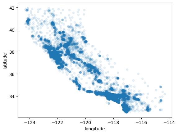
housing.plot(kind='scatter', x='longitude',y='latitude',alpha=0.1)

<Axes: xlabel='longitude', ylabel='latitude'>

%matplotlib inline
import matplotlib.pyplot as plt
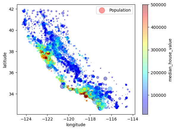
housing.plot(kind='scatter', x='longitude',y='latitude',alpha=0.4,
            s=housing['population']/100,label='Population',
            c='median_house_value',cmap=plt.get_cmap('jet'),colorbar=True)
plt.legend()

<matplotlib.legend.Legend at 0x26bee165690>

Method 1: Standard Correlation Coefficient

If the dataset is not too large, it is easy to calculate the standard correlation coefficient by using the corr() method.

The correlation coefficient ranges from -1 to 1, when it is close to -1, it means that there is a strong negative correlation, while when the coefficient is close to 1, it means that there is a strong positive correlation. Finally, coefficients close to zero mean that there is no linear correlation.

The correlation coefficient only measures linear correlations (“if x goes up, then y generally goes up or down”). It may completely miss out on nonlinear relationships.

import warnings
warnings.filterwarnings('ignore')

corr_matrix = housing.corr()
corr_matrix['median_house_value'].sort_values(ascending=False)

median_house_value    1.000000
median_income         0.688075
total_rooms           0.134153
housing_median_age    0.105623
households            0.065843
total_bedrooms        0.049686
population           -0.024650
longitude            -0.045967
latitude             -0.144160
Name: median_house_value, dtype: float64

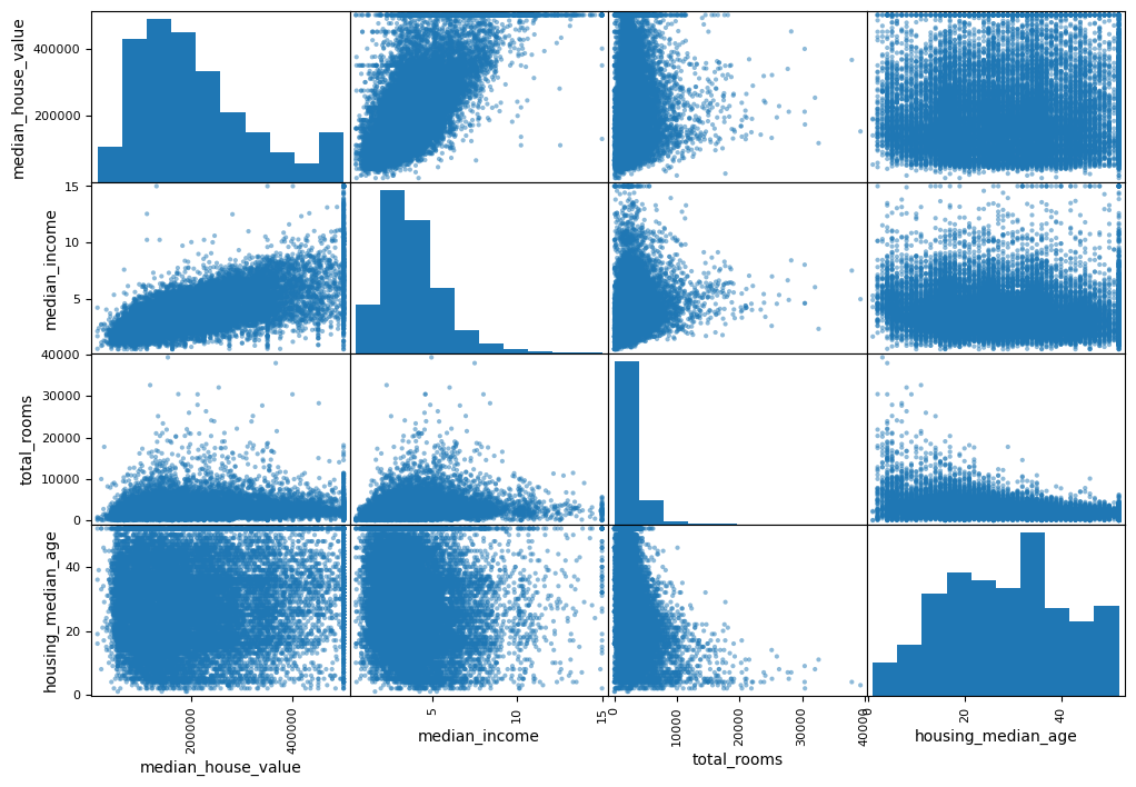
Method 2: Pandas scatter_matrix Function

Pandas’ scatter_matrix function plots every numerical attribute against every other numerical attribute, this could help to find out the correlation bettween each attribute visually.

from pandas.plotting import scatter_matrix

attributes = ['median_house_value', 'median_income', 'total_rooms', 'housing_median_age']
scatter_matrix(housing[attributes], figsize=(12,8))

array([[<Axes: xlabel='median_house_value', ylabel='median_house_value'>,
        <Axes: xlabel='median_income', ylabel='median_house_value'>,
        <Axes: xlabel='total_rooms', ylabel='median_house_value'>,
        <Axes: xlabel='housing_median_age', ylabel='median_house_value'>],
       [<Axes: xlabel='median_house_value', ylabel='median_income'>,
        <Axes: xlabel='median_income', ylabel='median_income'>,
        <Axes: xlabel='total_rooms', ylabel='median_income'>,
        <Axes: xlabel='housing_median_age', ylabel='median_income'>],
       [<Axes: xlabel='median_house_value', ylabel='total_rooms'>,
        <Axes: xlabel='median_income', ylabel='total_rooms'>,
        <Axes: xlabel='total_rooms', ylabel='total_rooms'>,
        <Axes: xlabel='housing_median_age', ylabel='total_rooms'>],
       [<Axes: xlabel='median_house_value', ylabel='housing_median_age'>,
        <Axes: xlabel='median_income', ylabel='housing_median_age'>,
        <Axes: xlabel='total_rooms', ylabel='housing_median_age'>,
        <Axes: xlabel='housing_median_age', ylabel='housing_median_age'>]],
      dtype=object)

Reference:

Aurelien Geron, Hands-On Machine Learning with Scikit-Learn & TensorFlow