Imputation of missing values using Scikit-Learn

Data Preparation

The widely used dataset: California Housing Prices to note down two ways to handle missing values in dataset by using Scikit-Learn. One type of imputation algorithm is univariate, and the other is multivariate imputation.

The first step is to download the data from Kaggle and read it by using Pandas.

import pandas as pd

housing = pd.read_csv('housing.csv')
housing.head()

	longitude	latitude	housing_median_age	total_rooms	total_bedrooms	population	households	median_income	median_house_value	ocean_proximity
0	-122.23	37.88	41.0	880.0	129.0	322.0	126.0	8.3252	452600.0	NEAR BAY
1	-122.22	37.86	21.0	7099.0	1106.0	2401.0	1138.0	8.3014	358500.0	NEAR BAY
2	-122.24	37.85	52.0	1467.0	190.0	496.0	177.0	7.2574	352100.0	NEAR BAY
3	-122.25	37.85	52.0	1274.0	235.0	558.0	219.0	5.6431	341300.0	NEAR BAY
4	-122.25	37.85	52.0	1627.0	280.0	565.0	259.0	3.8462	342200.0	NEAR BAY

housing.isnull().sum()

longitude               0
latitude                0
housing_median_age      0
total_rooms             0
total_bedrooms        207
population              0
households              0
median_income           0
median_house_value      0
ocean_proximity         0
dtype: int64

Univariate feature imputation

This method imputes values in the i-th feature dimension using only non-missing values in that feature dimension. Missing values can be imputed with a provided constant value, or using the statistics (mean, median or most frequent) of each column in which the missing values are located.

import numpy as np
from sklearn.impute import SimpleImputer
s_imp = SimpleImputer(missing_values=np.nan, strategy='median')
s_imp.fit(housing.drop("ocean_proximity", axis=1))

SimpleImputer(strategy='median')

In a Jupyter environment, please rerun this cell to show the HTML representation or trust the notebook.
On GitHub, the HTML representation is unable to render, please try loading this page with nbviewer.org.

s_imp.statistics_

array([-1.1849e+02,  3.4260e+01,  2.9000e+01,  2.1270e+03,  4.3500e+02,
        1.1660e+03,  4.0900e+02,  3.5348e+00,  1.7970e+05])

housing.drop("ocean_proximity", axis=1).median().values

array([-1.1849e+02,  3.4260e+01,  2.9000e+01,  2.1270e+03,  4.3500e+02,
        1.1660e+03,  4.0900e+02,  3.5348e+00,  1.7970e+05])

# After transform by the imputer, the result is a plain Numpy array, therefore it needs to be put back into a Pandas DataFrame.
housing_s = pd.DataFrame(s_imp.transform(housing.drop("ocean_proximity", axis=1)), columns=housing.drop("ocean_proximity", axis=1).columns)
housing_s.isnull().sum()

longitude             0
latitude              0
housing_median_age    0
total_rooms           0
total_bedrooms        0
population            0
households            0
median_income         0
median_house_value    0
dtype: int64

housing_s['total_bedrooms'].median()

435.0

Multivariate feature imputation

As its names stands, multivariate imputation algorithms use the entire set of available feature dimensions to estimate the missing values. This algorithm models each feature with missing values as a function of other features, and uses that estimate for imputation.

from sklearn.experimental import enable_iterative_imputer
from sklearn.impute import IterativeImputer
m_imp = IterativeImputer(max_iter=10, random_state=0)
m_imp.fit(housing.drop("ocean_proximity", axis=1))

IterativeImputer(random_state=0)

In a Jupyter environment, please rerun this cell to show the HTML representation or trust the notebook.
On GitHub, the HTML representation is unable to render, please try loading this page with nbviewer.org.

housing_m = pd.DataFrame(m_imp.transform(housing.drop("ocean_proximity", axis=1)), columns=housing.drop("ocean_proximity", axis=1).columns)
housing_m.isnull().sum()

longitude             0
latitude              0
housing_median_age    0
total_rooms           0
total_bedrooms        0
population            0
households            0
median_income         0
median_house_value    0
dtype: int64

housing_m['total_bedrooms'].median()

435.0

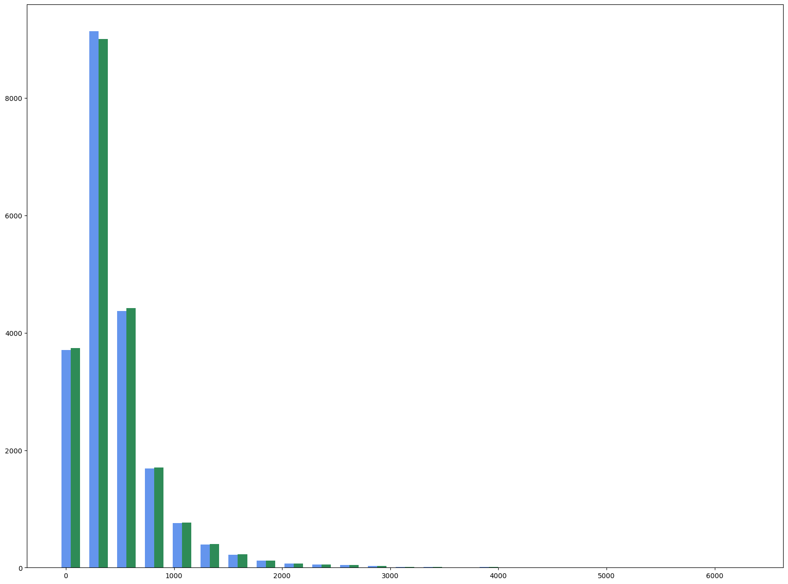
import matplotlib.pyplot as plt

fig, ax = plt.subplots(figsize=(20,15))

s_heights, s_bins = np.histogram(housing_s['total_bedrooms'], bins=25)
m_heights, m_bins = np.histogram(housing_m['total_bedrooms'], bins=s_bins)

width = (s_bins[1] - m_bins[0])/3

ax.bar(s_bins[:-1], s_heights, width=width, facecolor='cornflowerblue')
ax.bar(m_bins[:-1]+width, m_heights, width=width, facecolor='seagreen')

<BarContainer object of 25 artists>

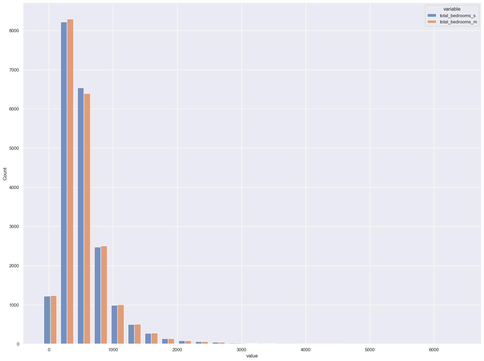
import seaborn as sns


df = pd.concat([housing_s['total_bedrooms'], housing_m['total_bedrooms']], axis=1, keys=['total_bedrooms_s', 'total_bedrooms_m'])
sns.set(rc={'figure.figsize':(20,15)})
sns.histplot(df.melt(), x='value', hue='variable', multiple='dodge', shrink=.75, bins=25);