Feature scaling using Scikit-Learn

Data Preparation

The widely used dataset: California Housing Prices to note down two ways to apply one of the most important transformations which is called feature scaling. This technique is used mainly when the input numerical attributes have very different scales which generate difficulty for the performance of machine learning algorithm.

For this dataset we can see the issue that the numerical attributes have very different scales, for example the total number of rooms ranges from about 2 to 39,320, while the median incomes only range from 0 to 15.

The first step is to download the data from Kaggle and read it by using Pandas.

import pandas as pd
import seaborn as sns
import matplotlib.pyplot as plt

housing = pd.read_csv('housing.csv')
housing.head()

	longitude	latitude	housing_median_age	total_rooms	total_bedrooms	population	households	median_income	median_house_value	ocean_proximity
0	-122.23	37.88	41.0	880.0	129.0	322.0	126.0	8.3252	452600.0	NEAR BAY
1	-122.22	37.86	21.0	7099.0	1106.0	2401.0	1138.0	8.3014	358500.0	NEAR BAY
2	-122.24	37.85	52.0	1467.0	190.0	496.0	177.0	7.2574	352100.0	NEAR BAY
3	-122.25	37.85	52.0	1274.0	235.0	558.0	219.0	5.6431	341300.0	NEAR BAY
4	-122.25	37.85	52.0	1627.0	280.0	565.0	259.0	3.8462	342200.0	NEAR BAY

housing[['total_rooms']].describe()

	total_rooms
count	20640.000000
mean	2635.763081
std	2181.615252
min	2.000000
25%	1447.750000
50%	2127.000000
75%	3148.000000
max	39320.000000

Normalization

Normalization is also called min-max scaling, it applies that values in the attributes to be shifted and rescaled to the range from 0 to 1 by default (it can be changed by identify the feature_range tuple). It is calculated by subtracting the min value and dividing by the max minus the min.

from sklearn.preprocessing import MinMaxScaler

m_scaler = MinMaxScaler(feature_range=(0,1))
housing_m_scaled = m_scaler.fit_transform(housing.drop(['longitude','latitude','ocean_proximity'], axis=1))

m_scaler.feature_names_in_

array(['housing_median_age', 'total_rooms', 'total_bedrooms',
       'population', 'households', 'median_income', 'median_house_value'],
      dtype=object)

m_scaler.scale_

array([1.96078431e-02, 2.54336436e-05, 1.55183116e-04, 2.80276914e-05,
       1.64446637e-04, 6.89645660e-02, 2.06184717e-06])

housing_m_scaled[0]

array([0.78431373, 0.02233074, 0.01986344, 0.00894083, 0.02055583,
       0.53966842, 0.90226638])

fig = plt.figure(figsize=(10,5))
sns.boxplot(housing_m_scaled[:,1])
plt.title('Box Plot: Total Rooms with MinMaxScaler', fontsize=15)
plt.ylabel('Scaled Total Rooms)', fontsize=14)
plt.show()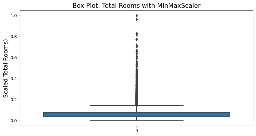

MaxAbsScaler

MaxAbsScaler is similar to MinMaxScaler except that the values are mapped across several ranges depending on whether negative or positive values are present. If only positive values are present the range is from 0 to 1, if only negative then -1 to 0, if both negative and positive values are present, the range would be -1 to 1.

from sklearn.preprocessing import MaxAbsScaler

ma_scaler = MaxAbsScaler()
housing_ma_scaled = ma_scaler.fit_transform(housing.drop(['longitude','latitude','ocean_proximity'], axis=1))

ma_scaler.feature_names_in_

array(['housing_median_age', 'total_rooms', 'total_bedrooms',
       'population', 'households', 'median_income', 'median_house_value'],
      dtype=object)

ma_scaler.scale_

array([5.20000e+01, 3.93200e+04, 6.44500e+03, 3.56820e+04, 6.08200e+03,
       1.50001e+01, 5.00001e+05])

housing_ma_scaled[0]

array([0.78846154, 0.02238047, 0.02001552, 0.00902416, 0.02071687,
       0.55500963, 0.90519819])

fig = plt.figure(figsize=(10,5))
sns.boxplot(housing_ma_scaled[:,1])
plt.title('Box Plot: Total Rooms with MaxAbsScaler', fontsize=15)
plt.ylabel('Scaled Total Rooms)', fontsize=14)
plt.show()

PowerTransformer

PowerTransformer applies a power transformation to each feature to make the data more Gaussian-like in order to stabilize variance and minimize skewness. By default, it applies zero-mean, unit variance normalization.

from sklearn.preprocessing import PowerTransformer

p_transformer = PowerTransformer(method='box-cox')
housing_p_scaled = p_transformer.fit_transform(housing.drop(['longitude','latitude','ocean_proximity'], axis=1))

p_transformer.feature_names_in_

array(['housing_median_age', 'total_rooms', 'total_bedrooms',
       'population', 'households', 'median_income', 'median_house_value'],
      dtype=object)

p_transformer.lambdas_

array([0.80939809, 0.22078296, 0.22469489, 0.23576758, 0.24492865,
       0.09085449, 0.12474767])

fig = plt.figure(figsize=(10,5))
sns.boxplot(housing_p_scaled[:,1])
plt.title('Box Plot: Total Rooms with PowerTransformer', fontsize=15)
plt.ylabel('Scaled Total Rooms)', fontsize=14)
plt.show()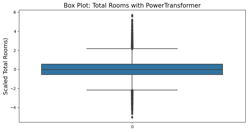

Standardization

Standardization removes the mean (so standardized values always have a zero mean) and scales the data to unit variance. Standardization does not bound values to a specific range, which may be a problem for some algorithms (e.g., neural networks often expect an input value ranging from 0 to 1). In addition, standardization is much less affected by outliers.

from sklearn.preprocessing import StandardScaler

s_scaler = StandardScaler()
housing_s_scaled = s_scaler.fit_transform(housing.drop(['longitude','latitude','ocean_proximity'], axis=1))

s_scaler.feature_names_in_

array(['housing_median_age', 'total_rooms', 'total_bedrooms',
       'population', 'households', 'median_income', 'median_house_value'],
      dtype=object)

s_scaler.scale_

array([1.25852527e+01, 2.18156240e+03, 4.21374759e+02, 1.13243469e+03,
       3.82320491e+02, 1.89977569e+00, 1.15392820e+05])

housing_s_scaled[0]

array([ 0.98214266, -0.8048191 , -0.97032521, -0.9744286 , -0.97703285,
        2.34476576,  2.12963148])

fig = plt.figure(figsize=(10,5))
sns.boxplot(housing_s_scaled[:,1])
plt.title('Box Plot: Total Rooms with StandardScaler', fontsize=15)
plt.ylabel('Scaled Total Rooms)', fontsize=14)
plt.show()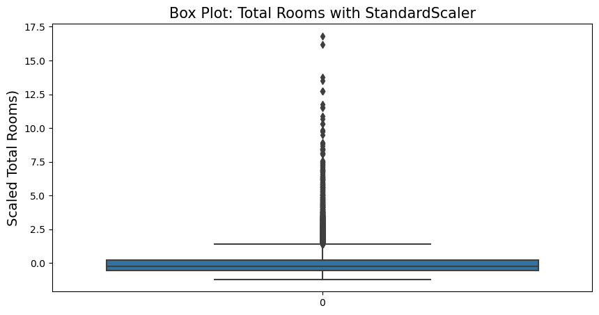

RobustScaler

The centering and scaling statistics of RobustScaler are based on the quantile range (defaults to IQR: interquantile Range). The IQR is the range between the 1st quanrtile (25th quantile) and the 3rd quartile (75th quantile). This provides good performance over outliers by defining the quantile_range.

from sklearn.preprocessing import RobustScaler

r_scaler = RobustScaler(quantile_range=(0.05,0.95))
housing_r_scaled = r_scaler.fit_transform(housing.drop(['longitude','latitude','ocean_proximity'], axis=1))

r_scaler.feature_names_in_

array(['housing_median_age', 'total_rooms', 'total_bedrooms',
       'population', 'households', 'median_income', 'median_house_value'],
      dtype=object)

r_scaler.scale_

array([2.000000e+00, 1.360000e+02, 3.100000e+01, 7.207050e+01,
       2.507050e+01, 5.601846e-01, 2.310415e+04])

housing_r_scaled[0]

array([  6.        ,  -9.16911765,  -9.87096774, -11.71075544,
       -11.28816737,   8.55146678,  11.81173079])

fig = plt.figure(figsize=(10,5))
sns.boxplot(housing_r_scaled[:,1])
plt.title('Box Plot: Total Rooms with RobustScaler', fontsize=15)
plt.ylabel('Scaled Total Rooms)', fontsize=14)
plt.show()

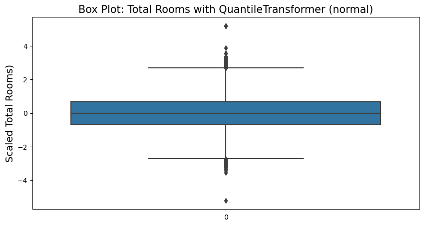
GuantileTransformer

QuantileTransformer applies a non-linear fransformation so that the probability density function of each feature will be mapped to a uniform or Gaussian distribution. In this case, all the data, including outliers, will be mapped to uniform or Gaussian distribution, making outliers indistinguishable from inliers.

But contrary to RobustScaler, QuantileTransformer will also automatically collapse any outlier by setting them to the a priori defined range boundaries (0 and 1). This can result in saturation artifacts for extreme values.

from sklearn.preprocessing import QuantileTransformer

gu_transformer = QuantileTransformer(output_distribution='uniform')
housing_gu_scaled = gu_transformer.fit_transform(housing.drop(['longitude','latitude','ocean_proximity'], axis=1))

gu_transformer.feature_names_in_

array(['housing_median_age', 'total_rooms', 'total_bedrooms',
       'population', 'households', 'median_income', 'median_house_value'],
      dtype=object)

gu_transformer.quantiles_[0]

array([1.0000e+00, 8.0000e+00, 1.0000e+00, 3.0000e+00, 1.0000e+00,
       4.9990e-01, 1.4999e+04])

fig = plt.figure(figsize=(10,5))
sns.boxplot(housing_gu_scaled[:,1])
plt.title('Box Plot: Total Rooms with QuantileTransformer (uniform)', fontsize=15)
plt.ylabel('Scaled Total Rooms)', fontsize=14)
plt.show()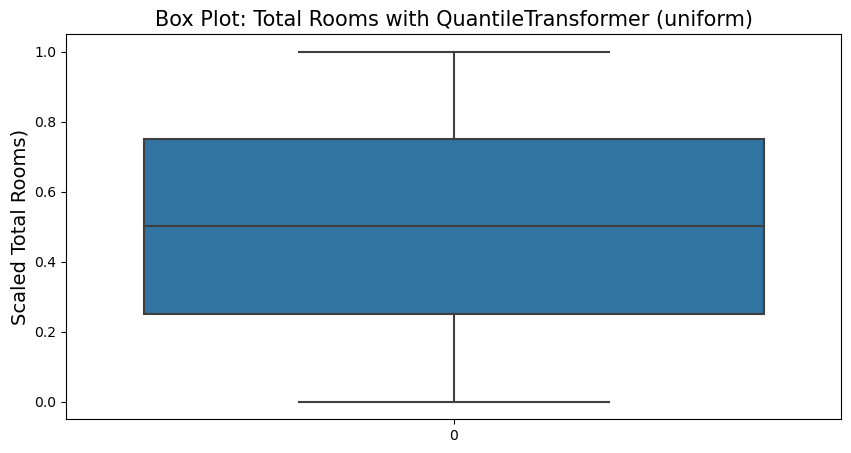

from sklearn.preprocessing import QuantileTransformer

gn_transformer = QuantileTransformer(output_distribution='normal')
housing_gn_scaled = gn_transformer.fit_transform(housing.drop(['longitude','latitude','ocean_proximity'], axis=1))

gn_transformer.feature_names_in_

array(['housing_median_age', 'total_rooms', 'total_bedrooms',
       'population', 'households', 'median_income', 'median_house_value'],
      dtype=object)

gn_transformer.quantiles_[0]

array([1.0000e+00, 2.0000e+00, 1.0000e+00, 5.0000e+00, 2.0000e+00,
       4.9990e-01, 1.4999e+04])

fig = plt.figure(figsize=(10,5))
sns.boxplot(housing_gn_scaled[:,1])
plt.title('Box Plot: Total Rooms with QuantileTransformer (normal)', fontsize=15)
plt.ylabel('Scaled Total Rooms)', fontsize=14)
plt.show()