Data preparation

Fetch MNIST dataset which contains a set of 70,000 small images of digits handwritten by high school students and employees of the US Census Bureau. RidgeClassifier is used for prediction whether the handwriten digit is 5 or not.

from sklearn.datasets import fetch_openml
from sklearn.linear_model import RidgeClassifier
from sklearn.metrics import confusion_matrix
import numpy as np
import warnings
warnings.filterwarnings('ignore')

mnist = fetch_openml('mnist_784', version=1)
X, y = mnist["data"], mnist["target"]
y = y.astype(np.uint8)
X_train, X_test, y_train, y_test = X[:60000], X[60000:], y[:60000], y[60000:]

y_train_5 = (y_train == 5)
y_test_5 = (y_test == 5)

ridge_clf = RidgeClassifier()
ridge_clf.fit(X_train, y_train_5)

RidgeClassifier()

In a Jupyter environment, please rerun this cell to show the HTML representation or trust the notebook.
On GitHub, the HTML representation is unable to render, please try loading this page with nbviewer.org.

Confusion matrix visualization

import itertools
import matplotlib.pyplot as plt

def plot_confusion_matrix(cm, classes, title='Confusion matrix', cmap=plt.cm.Blues):
    """
    This function prints and plots the confusion matrix.
    Normalization can be applied by setting `normalize=True`.
    """
    plt.imshow(cm, interpolation='nearest', cmap=cmap)
    plt.title(title)
    plt.colorbar()
    tick_marks = np.arange(len(classes))
    plt.xticks(tick_marks, classes, rotation=0)
    plt.yticks(tick_marks, classes)

    thresh = cm.max() / 2.
    for i, j in itertools.product(range(cm.shape[0]), range(cm.shape[1])):
        plt.text(j, i, cm[i, j],
                 horizontalalignment="center",
                 color="white" if cm[i, j] > thresh else "black")

    # plt.tight_layout()
    plt.ylabel('True label')
    plt.xlabel('Predicted label')

from sklearn.model_selection import cross_val_predict
import numpy as np
y_train_5_pred = cross_val_predict(ridge_clf, X_train, y_train_5, cv=3)
cm = confusion_matrix(y_train_5, y_train_5_pred)

plt.figure()
plot_confusion_matrix(cm , classes=["5","Non-5"], title='Confusion matrix')
plt.show()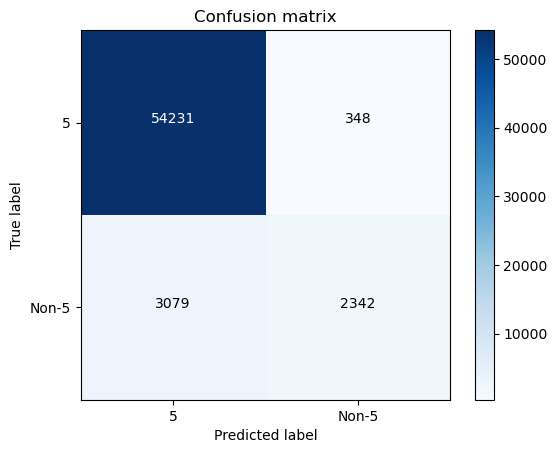

Confusion matrix

Accuracy

Accuracy is the ratio of total correct instances to the total instances. the potential risk to use this is for skewed dataset it actually cannot reflect the model’s performance perfectly.

from sklearn.metrics import accuracy_score
accuracy_score(y_train_5, y_train_5_pred)

0.9428833333333333

y_train_5.describe()

count     60000
unique        2
top       False
freq      54579
Name: class, dtype: object

As we can see this dataset is skewed where non-5 digits occupied most of it, if we predict all digits as non-5, we could still get pretty good accuracy.

y_train_5_new_pred = np.zeros((len(y_train_5), 1), dtype=bool)
accuracy_score(y_train_5, y_train_5_new_pred)

0.90965

Precision

Precision is defined as the ratio of true positive predictions to the total number of positive predictions made by the model, it could be used to measure how accurate a model’s positive predictions are (the ability of the model not to label as positive a sample that is negative).

Precision = TP/(TP+FP)

from sklearn.metrics import precision_score
precision_score(y_train_5, y_train_5_pred)

0.8706319702602231

Recall

Recall is the ratio of the number of true positive instances to the sum of true positive and false negative instanes, it measures the effectiveness of the model in identifying all relevant instances from a dataset (the ability of the classifier to find all the positive samples).

Recall = TP/(TP+FN)

from sklearn.metrics import recall_score
recall_score(y_train_5, y_train_5_pred)

0.432023611879727

F1-Score

F1-Score is the harmonic mean of precision and recall, it is used to evaluate the overall performance. The relative contribution of precision and recall to the F1 score are equal.

F-Score = 2 * Precision * Recall / (Precision + Recall) = 2 * TP / (2 * TP + FN + FP)

from sklearn.metrics import f1_score
f1_score(y_train_5, y_train_5_pred)

0.5774873628405869

Specificity

Specificity is also known as the True Negative Rate, it measures the ability of a model to correctly identify negative instances.

Specificity = TN/(TN+FP)

There is no direct way in sklearn.metrics to calculate the Specificity, here below are two indirect ways.

# Method 1
from sklearn.metrics import confusion_matrix
tn, fp, fn, tp = confusion_matrix(y_train_5, y_train_5_pred).ravel()

specificity = tn/(tn+fp)
specificity

0.9936239212884076

# Method 2, specificity is the recall of the negative class
from sklearn.metrics import recall_score
recall_score(y_train_5, y_train_5_pred, pos_label=0)

0.9936239212884076

Type 1 and Type 2 error

Type 1 error occurs when the model predicts a positive instance, but it is actually negative. Precision is affected by false positives, as it is the ratio of true positives to the sum of true positives and false positives.

Type 1 Error = FP/(TP+FP)

Type 2 error occurs when the model fails to predict a positive instance. Recall is directly affected by false negatives, as it is the ratio of true positives to the sum of true positives and false negatives.

Type 2 Error = FN/(TP+FN)

Precision emphasizes minimizing false positives, while recall focuses on minimizing false negatives.