Calculate Capital Asset Pricing Model (CAPM) with Python

Capital Asset Pricing Model (CAPM)

CAPM is one of the most commonly used formula in finance, which describes the relationship betwwen systematic risk and expected return for assets, particularly stocks. The model is based on the relationship between an asset’s beta, the risk-free rate (typically the Treasury bill rate) and the equity risk premium.

The CAPM formula is as below:

$$r_i = r_f + \beta_i(r_m - r_f)$$

Where:

• $r_i$ is the expected return of a security
• $r_f$ is the risk free rate
• $\beta_i$ is the beta of the security relative to the market
• $r_m$ is the market return which includes all securities in the market. A good representation of the U.S. market portfolio is the S&P 500.

The goal of the CAPM formula is to gauge whether the current price of a stock is consistent with its likely return.

The beta is a measure of how much risk the investment will add to a portfolio that looks like the market, or a measure of a portfolio’s volatility in relation to the overall market. If beta is less than 1, it indicates the portforlio is less volatile than the market, which means it reduces the risk of a portfolio. On the other hand, if a portforlio is riskier than the market, it will have a betwa greater than 1.

Load the list of S&P 500 companies from Wikepedia

S&P 500 is a stock market index tracking the stock performance of 500 of the largest companies listed on stock exchanges in the United States.

# Get the list of S&P 500 stocks from Wikepedia
import pandas as pd

def load_data(url):
    html = pd.read_html(url, header=0)
    return html

# Load the list of S&P 500 companies
url = 'https://en.wikipedia.org/wiki/List_of_S%26P_500_companies'
df = load_data(url)[0]
df.head()

	Symbol	Security	GICS Sector	GICS Sub-Industry	Headquarters Location	Date added	CIK	Founded
0	MMM	3M	Industrials	Industrial Conglomerates	Saint Paul, Minnesota	1957-03-04	66740	1902
1	AOS	A. O. Smith	Industrials	Building Products	Milwaukee, Wisconsin	2017-07-26	91142	1916
2	ABT	Abbott	Health Care	Health Care Equipment	North Chicago, Illinois	1957-03-04	1800	1888
3	ABBV	AbbVie	Health Care	Biotechnology	North Chicago, Illinois	2012-12-31	1551152	2013 (1888)
4	ACN	Accenture	Information Technology	IT Consulting & Other Services	Dublin, Ireland	2011-07-06	1467373	1989

Retrieve the latest stock price using yfinance

We retrieve the latest year’s stock price using yfinance.

import warnings
warnings.filterwarnings('ignore')
import yfinance as yf

data = yf.download(
            # tickers list
            tickers = list(df['Symbol']) + ['^GSPC'],
            # valid periods: 1d, 5d, 1mo, 3mo, 6mo, 1y, 5y, 10y, ytd, max
            period = '1y',
            # valid intervals: 1m, 2m, 5m, 15m, 15m, 30m, 60m, 90m, 1h, 1d, 5d, 1wk, 1mo, 3mo
            interval = '1d',
            # group by ticker
            group_by = 'ticker',
            # adjust all OHLC automatically
            auto_adjust = True,
            # download pre/post regular market hours data
            prepost = True,
            # use threads for mass downloading
            threads = True,
            # proxy URL scheme when downloading
            proxy = None
            )

[*********************100%%**********************]  504 of 504 completed

2 Failed downloads:
['BF.B']: Exception('%ticker%: No price data found, symbol may be delisted (period=1y)')
['BRK.B']: Exception('%ticker%: No data found, symbol may be delisted')

data['^GSPC'].head()

Price	Open	High	Low	Close	Volume
Date
2023-02-27	3992.360107	4018.050049	3973.550049	3982.239990	3836950000
2023-02-28	3977.189941	3997.500000	3968.979980	3970.149902	5043400000
2023-03-01	3963.340088	3971.729980	3939.050049	3951.389893	4249480000
2023-03-02	3938.679932	3990.840088	3928.159912	3981.350098	4244900000
2023-03-03	3998.020020	4048.290039	3995.169922	4045.639893	4084730000

# Get the available tickers
tickers_unavailable = ['BF.B', 'BRK.B']
tickers = [ticker for ticker in list(df['Symbol']) + ['^GSPC'] if ticker not in tickers_unavailable]
print('Number of available tickers: ', len(tickers))

Number of available tickers:  502

# Use Close as the price for each stock and create a new dataframe to store this data.
import numpy as np
stock = pd.DataFrame(columns = ['Date'], data = data['MMM'].index)
for i in range(0,len(tickers)):
    ticker = tickers[i]
    stock = stock.join(
             pd.Series(
                 data[ticker]['Close'].to_list(), 
                 name=ticker,
                 index=stock.index))

stock = stock.set_index('Date')
stock.head()

	MMM	AOS	ABT	ABBV	ACN	ADBE	AMD	AES	AFL	A	...	GWW	WYNN	XEL	XYL	YUM	ZBRA	ZBH	ZION	ZTS	^GSPC
Date
2023-02-27	101.759285	64.206650	97.783730	148.282318	262.200623	322.320007	78.769997	23.996420	66.643791	141.154373	...	668.472412	104.074387	63.236515	101.250412	124.182861	296.230011	122.350578	47.859604	163.987595	3982.239990
2023-02-28	101.261154	64.511368	99.694916	147.917068	261.511230	323.950012	78.580002	23.803526	66.565651	140.945908	...	661.946350	107.271660	62.433975	101.349144	124.761726	300.250000	122.916191	48.078060	165.503891	3970.149902
2023-03-01	103.582634	65.631935	98.822639	149.233841	259.581085	323.380005	78.290001	23.755301	66.536346	136.518066	...	664.501221	111.082634	61.176975	99.808891	123.819832	302.339996	121.139977	47.907097	166.068771	3951.389893
2023-03-02	103.291267	66.487114	100.586800	148.378433	261.225677	333.500000	80.440002	23.764944	65.989365	140.648071	...	677.860413	112.260574	62.211575	100.954201	126.253059	306.059998	122.042961	45.884064	167.069748	3981.350098
2023-03-03	104.569481	66.968750	102.370560	149.993103	265.105774	344.040009	81.519997	24.208611	66.848907	142.891754	...	690.823425	114.656044	62.946434	102.603035	127.224380	309.450012	125.248100	46.757858	169.031982	4045.639893

5 rows × 502 columns

Normalize and visualize the stock data

# Normalize stock data based on initial price
def normalize(df):
    x = df.copy()
    for i in x.columns:
        x[i] = x[i]/x[i][0]
    return x

stock_normalized = normalize(stock)
stock_normalized.head()

	MMM	AOS	ABT	ABBV	ACN	ADBE	AMD	AES	AFL	A	...	GWW	WYNN	XEL	XYL	YUM	ZBRA	ZBH	ZION	ZTS	^GSPC
Date
2023-02-27	1.000000	1.000000	1.000000	1.000000	1.000000	1.000000	1.000000	1.000000	1.000000	1.000000	...	1.000000	1.000000	1.000000	1.000000	1.000000	1.000000	1.000000	1.000000	1.000000	1.000000
2023-02-28	0.995105	1.004746	1.019545	0.997537	0.997371	1.005057	0.997588	0.991962	0.998827	0.998523	...	0.990237	1.030721	0.987309	1.000975	1.004661	1.013570	1.004623	1.004565	1.009246	0.996964
2023-03-01	1.017918	1.022198	1.010625	1.006417	0.990009	1.003289	0.993906	0.989952	0.998388	0.967154	...	0.994059	1.067339	0.967431	0.985763	0.997077	1.020626	0.990105	1.000992	1.012691	0.992253
2023-03-02	1.015055	1.035518	1.028666	1.000648	0.996282	1.034686	1.021201	0.990354	0.990180	0.996413	...	1.014044	1.078657	0.983792	0.997074	1.016671	1.033184	0.997486	0.958722	1.018795	0.999777
2023-03-03	1.027616	1.043019	1.046908	1.011537	1.011080	1.067386	1.034912	1.008843	1.003078	1.012308	...	1.033436	1.101674	0.995413	1.013359	1.024492	1.044627	1.023682	0.976980	1.030761	1.015921

5 rows × 502 columns

# Plot the normalized price of several selected stocks
import plotly.express as px
fig = px.line(title = 'Normalized Prices')
for ticker in ['AMD','AAPL','GOOG', 'TSLA','IBM']:
    fig.add_scatter(x=stock_normalized.index, y=stock_normalized[ticker], name=ticker)
fig.show()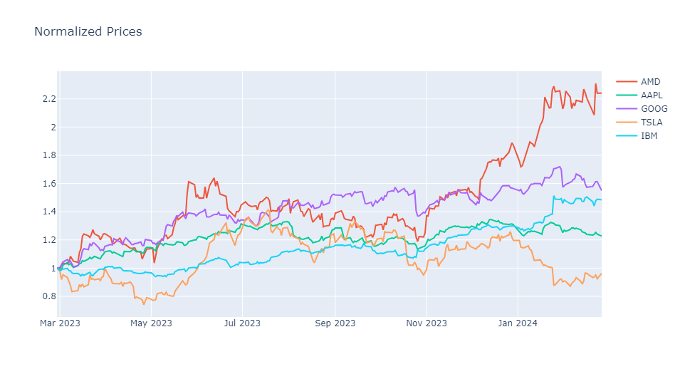

Calculate the daily return

The daily return for each stock is calculated as follows:

• Loop to each row of the stock normalized price
• Calculate the percentage change from the previous day
• The first row is set to 0 as there is no previous value

def daily_return(df):
    df_daily_return = df.copy()
    for i in df.columns:
        for j in range(1, len(df)):
            df_daily_return[i][j] = ((df[i][j]- df[i][j-1])/df[i][j-1]) * 100
        df_daily_return[i][0] = 0
    return df_daily_return

stock_daily_return = daily_return(stock_normalized)
stock_daily_return.head()

	MMM	AOS	ABT	ABBV	ACN	ADBE	AMD	AES	AFL	A	...	GWW	WYNN	XEL	XYL	YUM	ZBRA	ZBH	ZION	ZTS	^GSPC
Date
2023-02-27	0.000000	0.000000	0.000000	0.000000	0.000000	0.000000	0.000000	0.000000	0.000000	0.000000	...	0.000000	0.000000	0.000000	0.000000	0.000000	0.000000	0.000000	0.000000	0.000000	0.000000
2023-02-28	-0.489519	0.474589	1.954503	-0.246320	-0.262925	0.505710	-0.241202	-0.803845	-0.117251	-0.147686	...	-0.976265	3.072104	-1.269108	0.097513	0.466139	1.357050	0.462289	0.456452	0.924641	-0.303600
2023-03-01	2.292567	1.737008	-0.874946	0.890210	-0.738074	-0.175955	-0.369052	-0.202598	-0.044023	-3.141518	...	0.385963	3.552638	-2.013327	-1.519749	-0.754955	0.696085	-1.445062	-0.355595	0.341309	-0.472526
2023-03-02	-0.281289	1.302992	1.785178	-0.573200	0.633556	3.129444	2.746202	0.040595	-0.822080	3.025244	...	2.010409	1.060418	1.691158	1.147502	1.965136	1.230403	0.745406	-4.222826	0.602748	0.758219
2023-03-03	1.237485	0.724405	1.773354	1.088211	1.485343	3.160422	1.342608	1.866895	1.302548	1.595246	...	1.912342	2.133848	1.181226	1.633250	0.769345	1.107631	2.626238	1.904353	1.174500	1.614774

5 rows × 502 columns

# Plot the daily return for the selected stocks
fig = px.line(title = 'Daily Return')
for ticker in ['AMD','AAPL','GOOG', 'TSLA','IBM']:
    fig.add_scatter(x=stock_daily_return.index, y=stock_daily_return[ticker], name=ticker)
fig.show()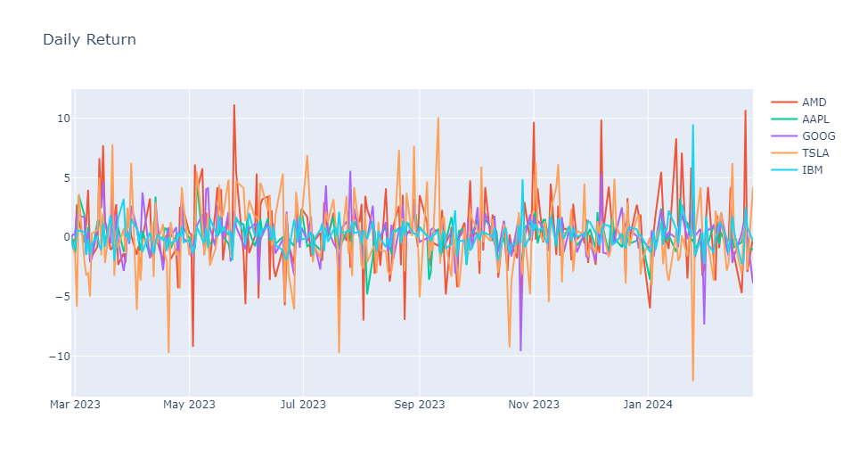

Calculate Beta for AAPL

Beta is the slope of the line regression line, or the market return vs. stock return, which could be calculated using np.polyfit

# S&P 500 has ticker symbol ^GSPC

beta, alpha = np.polyfit(stock_daily_return['^GSPC'], stock_daily_return['AAPL'], 1)
beta

1.0716621967198638

Calculate CAPM for AAPL

# Daily return for the market
stock_daily_return['^GSPC'].mean()

0.09994347738081993

# Annual return for the market would be the daily return multiply the number of trading days in a year
r_m = stock_daily_return['^GSPC'].mean() * 252
print('Return of the market: ', r_m)

Return of the market:  25.185756299966624

# Expected return could be calculated using CAPM formula
# Assume the risk free rate rate is 0
r_f = 0
r_e_AAPL = r_f + beta * (r_m - r_f)
print('Expected return: ', r_e_AAPL)

Expected return:  26.99062292247338

Apparently this is not realistic.

• The markets are very competitive and efficient, investors who work in the markets are rational and risk-averse. Everything can change very fast.

Reference:

https://www.investopedia.com/terms/c/capm.asp

https://www.mlq.ai/capital-asset-pricing-model-python/