Risk-adjusted performance metrics calculation in Python

Publish Date: 2024-03-06

Update Date: 2024-03-23

Word Count: 1.1k

Read Times: 7 Min

Read Count:

Sharpe Ratio

It is virtually impossible to increase return without also increasing risk, therefore it shall exist a trade-off between risk and return which encourages us to find a metric so that by using it we can maximize the return while minimize the risk.

The Sharpe Ratio, developed by Nobel Prize winner William Sharpe, helps investors evaluate the return of an investment compared to its risk relative to a risk-free asset. It has three key metrics: the annual return of the investment, the prevailing risk-free rate, and the standard deviation of the investment’s returns.

Shape Ratio = (r_portfolio - r_rf) / std_portfolio

Where:

r_portfolio is annual return of the portfolio
r_rf is the risk-free rate - usually the rate offered by short-term Treasury bills.
std_portfolio is the standard deviation of the portfolio’s return.

Now is the moment to estimate the Sharpe Ratio for S&P 500 (^GSPC) by using Python.

import numpy as np
import pandas as pd
import yfinance as yf

sp500 = yf.Ticker('^GSPC')
data_sp500 = sp500.history(interval='1d', start='2023-03-06', end='2024-03-06')
data_sp500.head()

	Open	High	Low	Close	Volume	Dividends	Stock Splits
Date
2023-03-06 00:00:00-05:00	4055.149902	4078.489990	4044.610107	4048.419922	4000870000	0.0	0.0
2023-03-07 00:00:00-05:00	4048.260010	4050.000000	3980.310059	3986.370117	3922500000	0.0	0.0
2023-03-08 00:00:00-05:00	3987.550049	4000.409912	3969.760010	3992.010010	3535570000	0.0	0.0
2023-03-09 00:00:00-05:00	3998.659912	4017.810059	3908.699951	3918.320068	4445260000	0.0	0.0
2023-03-10 00:00:00-05:00	3912.770020	3934.050049	3846.320068	3861.590088	5518190000	0.0	0.0

sp500_close = data_sp500['Close']
# Daily return is estimated as the log difference from the closing price
sp500_dr = np.log(sp500_close).diff().dropna()

Consdier 260 weekdays in a 52-week year, but generally markets are closed for about 8 days each year for holidays, therefore to calculate the yearly mean return we could use the average daily return to multiply 252.

sp500_meanreturn = np.mean(sp500_dr)*251
sp500_volatility = np.std(sp500_dr) * np.sqrt(251)

# Calculate the Sharpe Ratio of S&P500
# risk-free rate is using short-term Threasury yields ~5% (https://www.bloomberg.com/markets/rates-bonds/government-bonds/us)
rfr = 0.05
sp500_sharpe_ratio = (sp500_meanreturn - rfr)/sp500_volatility 
print('The estimated Sharpe Ratio for S&P 500 is: ', sp500_sharpe_ratio)

The estimated Sharpe Ratio for S&P 500 is:  1.4460114773564745

print('S&P 500 total return is: ', sp500_close[-1]/sp500_close[0] - 1)
print('S&P 500 volatility is: ', sp500_volatility)

S&P 500 total return is:  0.254477055332641
S&P 500 volatility is:  0.1222111992429432

The above result implies that to achieve 25.45% - 5% = 20.45% yearly return, the volatility would be 12.22%, this also informs that:

Maximum gain: Volatility + Excess Return = 12.22% + 20.45% = 32.67%
Maximum loss: -Volatility + Excess Return = -12.22% + 20.45% = 8.23%

In this case, in a year range, the excess return could be range between 8.23% to 32.67%

Sortino Ratio

When calculating Sharpe Ratio, the standard deviation is used as the volatility, while it does not differentiate upward deviations from downward deviations, and in fact we actually seek upward deviations.

The Sortino Ratio is very similar to the Sharpe Ratio, the only difference being that where the Sharpe Ratio uses all the observations for calculating the standard deviation while the Sortino Ratio only considers the downward deviations.

def sortino_ratio(series, td, rfr):
    mean = series.mean() * td - rfr
    std_neg = series[series<0].std() * np.sqrt(td)
    return mean/std_neg

sp500_sortino_ratio = sortino_ratio(sp500_dr, 252, 0.05)

print('The estimated Sortino Ratio for S&P 500 is: ', sp500_sortino_ratio)

The estimated Sortino Ratio for S&P 500 is:  2.318163296302093

Calmar Ratio

Before talking about the Carmar Ratio, we need to understand the Max Drawdown, which quantifies the steepest decline from peak to trough observed for an investment.

Max Drawdown is useful as it doesn’t rely on the underlying returns being normally distributed (which is not realistic in the markets).

The Max Drawdown should be interpreted as: numbers closer to zero are preferable.

def max_drawdown(series):
    compound_return = series.cumprod()
    peak = compound_return.expanding(min_periods=1).max()
    drawdown = compound_return/peak - 1
    return drawdown.min()

sp500_max_drawdown = max_drawdown(sp500_dr)

print('The estimated Max Drawdown for S&P 500 is: ', sp500_max_drawdown)

The estimated Max Drawdown for S&P 500 is:  -1.0145839694360674

The Carmar Ratio is then calculated as the average return divided by the Max Drawdown.

def carmar_ratio(series, td):
    max_dd = abs(max_drawdown(series))
    return series.mean() * td / max_dd

sp500_carmar_ratio = carmar_ratio(sp500_dr, 252)

print('The estimated Carmar Ratio for S&P 500 is: ', sp500_carmar_ratio)

The estimated Carmar Ratio for S&P 500 is:  0.22435014327283942

Omega Ratio

The Sharpe Ratio and Sortino Ratio works well if the return is in normal distribution, while this is not realistic in the markets. The Sharpe Ratio could hide some important information about the patterns of the returns, for example two different return distributions could have the same mean and standard deviation, but differ significantly in other aspects.

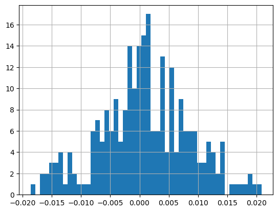
Omega Ratio is the probability-weighted ratio of gains over losses at a given level of expected return (known as threshold). It does this by adding up the area under the distribution around the threshold, the area above the threshold measures the weight of the gains, while the area below the threshold measures the weight of the losses. The Omega Ratio is the positive area divided by the negative area.

def omega_ratio(series, td, threshold):
    # calculate daily threshold
    dailyThreshold = (threshold+1)**np.sqrt(1/td)-1
    # calculate the excess return
    excess_return = series - dailyThreshold
    # get sum of all values excess return above 0
    positiveSum = sum(excess_return[excess_return > 0])
    # get sum of all values excess return below 0
    negativeSum = sum(excess_return[excess_return < 0])
    
    return positiveSum/(-negativeSum)

sp500_dr.hist(bins=50)

<Axes: >

S&P500 Daily Return

sp500_omega_ratio = omega_ratio(sp500_dr, 252, 0.005)

print('The estimated Omega Ratio with threshold 0.5% for S&P 500 is: ', sp500_omega_ratio)

The estimated Omega Ratio with threshold 0.5% for S&P 500 is:  1.2180141953898103

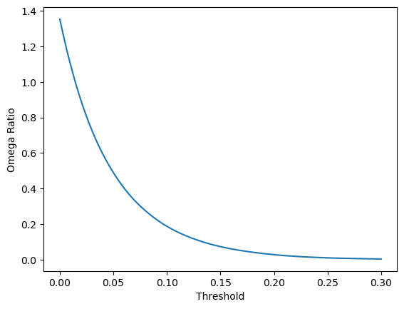
It has better view to plot the Omega Ratio curve with changing thresholds.

import matplotlib.pyplot as plt
omega_ratios = []
thresholds = np.linspace(0,0.3,100)
for t in thresholds:
    val = round(omega_ratio(sp500_dr, 252, t), 10)
    omega_ratios.append(val)

plt.plot(thresholds, omega_ratios)
plt.ylabel("Omega Ratio")
plt.xlabel("Threshold")