Geospatial interpolation - Thiessen Polygons

Thiessen polygon, also called Voronoi diagram, is a partition of a plane into regions close to each of a given set of objects. Thiessen polygons are be constructed around each sampled point so all the space within a specific polygon is closest in distance to that sampled point (comparing to other sampled points).

scipy package offers Voronoi() function to create Thiessen polygons.

Data Preparation

National Land Survey of Finland (https://www.maanmittauslaitos.fi/en) provides the latest shapefile for the Finnish administration boarders, which includes the municipalities.

OpenCellID (https://opencellid.org/) is a collaborative community project that collects GPS positions of cell towers and their corresponding location area identity.

In this section, we will map the collected cell towers to each municipalities and provinces, and export the merged dataframe.

When download the dataset which contains the cell towers’ GPS information, it is in EPSG:4326 coded. While the shapefile for Finnish municipality and province, the CRS is EPSG:3067.

import pandas as pd
import geopandas as gpd
import matplotlib.pyplot as plt
import contextily as ctx
from geopandas import GeoDataFrame
from shapely.geometry import Point
import pyproj
import warnings
warnings.filterwarnings('ignore')

# load DNA LTE cell towers list downloaded from OpenCellID
dna_cell_tower = pd.read_csv('dna_lte.csv')
dna_cell_tower.head()

	Unnamed: 0	MCC	MCNC	eNB_ID	Longitude	Latitude
0	7489	244	12	2	24.607037	60.731043
1	7490	244	12	3	24.400345	60.997403
2	7491	244	12	4	24.613302	60.706910
3	7492	244	12	5	24.499218	60.912731
4	7493	244	12	6	24.510986	60.884484

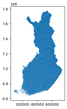
# load Finland municipality boundary spatial data downloaded from National Land Survey of Finland
finland_municipality = gpd.GeoDataFrame.from_file('kunta1000k_2023Polygon.shp')
finland_municipality.plot()

<Axes: >

# load Finland province boundary spatial data downloaded from National Land Survey of Finland
finland_province = gpd.GeoDataFrame.from_file('maakunta1000k_2023Polygon.shp')
finland_province.plot()

<Axes: >

# create a function to map each municipality to province
def municipality2province(municipality, province):
    for ind in province.index:
        if province['geometry'][ind].contains(municipality):
            return province['name'][ind]
        
finland_municipality['province'] = finland_municipality['geometry'].apply(lambda x: municipality2province(x, finland_province))

finland_municipality.head()

	kunta	vuosi	nimi	namn	name	geometry	province
0	005	2023	Alajärvi	Alajärvi	Alajärvi	POLYGON ((366787.924 7001300.583, 364487.590 6...	South Ostrobothnia
1	009	2023	Alavieska	Alavieska	Alavieska	POLYGON ((382543.364 7120022.976, 382899.505 7...	North Ostrobothnia
2	010	2023	Alavus	Alavo	Alavus	POLYGON ((343298.204 6961570.195, 343831.847 6...	South Ostrobothnia
3	016	2023	Asikkala	Asikkala	Asikkala	POLYGON ((436139.680 6798279.085, 435714.468 6...	Päijät-Häme
4	018	2023	Askola	Askola	Askola	POLYGON ((426631.036 6720528.076, 428821.749 6...	Uusimaa

Data Wrangling

In the following we will transform the GPS (WGS84 or EPSG:4326) to EPSG3067, and then merge two datasets and count the number of cell towers per municipality.

# create several functions to transform the projections
wgs84 = pyproj.Proj(projparams = 'epsg:4326')
finProj = pyproj.Proj(projparams = 'epsg:3067')

def crs_transformer(x, y):
    return pyproj.transform(wgs84,finProj, y, x)

def transformed_x(x,y):
    return crs_transformer(x,y)[0]

def transformed_y(x,y):
    return crs_transformer(x,y)[1]

# transform the cell tower's coordinates to EPSG3067
dna_cell_tower['Proj_Lon'] = dna_cell_tower.apply(lambda x: transformed_x(x['Longitude'], x['Latitude']), axis=1)
dna_cell_tower['Proj_Lat'] = dna_cell_tower.apply(lambda x: transformed_y(x['Longitude'], x['Latitude']), axis=1)

dna_cell_tower.head()

	Unnamed: 0	MCC	MCNC	eNB_ID	Longitude	Latitude	Proj_Lon	Proj_Lat
0	7489	244	12	2	24.607037	60.731043	369501.553119	6.735208e+06
1	7490	244	12	3	24.400345	60.997403	359409.547832	6.765288e+06
2	7491	244	12	4	24.613302	60.706910	369745.411927	6.732509e+06
3	7492	244	12	5	24.499218	60.912731	364394.910111	6.755654e+06
4	7493	244	12	6	24.510986	60.884484	364913.374089	6.752485e+06

# create a GeoDataFrame with each cell location as a Point
dna_cell_tower_gdf = gpd.GeoDataFrame(dna_cell_tower, geometry=gpd.points_from_xy(dna_cell_tower['Proj_Lon'], dna_cell_tower['Proj_Lat'], crs='EPSG:3067'))
dna_cell_tower_gdf.head()

	Unnamed: 0	MCC	MCNC	eNB_ID	Longitude	Latitude	Proj_Lon	Proj_Lat	geometry
0	7489	244	12	2	24.607037	60.731043	369501.553119	6.735208e+06	POINT (369501.553 6735208.061)
1	7490	244	12	3	24.400345	60.997403	359409.547832	6.765288e+06	POINT (359409.548 6765288.274)
2	7491	244	12	4	24.613302	60.706910	369745.411927	6.732509e+06	POINT (369745.412 6732508.849)
3	7492	244	12	5	24.499218	60.912731	364394.910111	6.755654e+06	POINT (364394.910 6755653.753)
4	7493	244	12	6	24.510986	60.884484	364913.374089	6.752485e+06	POINT (364913.374 6752484.785)

# merge cell tower dataframe and municipality dataframe
merge_gdf = dna_cell_tower_gdf.sjoin(finland_municipality[['kunta','name','geometry','province']], how='left')
merge_gdf.head()

	Unnamed: 0	MCC	MCNC	eNB_ID	Longitude	Latitude	Proj_Lon	Proj_Lat	geometry	index_right	kunta	name	province
0	7489	244	12	2	24.607037	60.731043	369501.553119	6.735208e+06	POINT (369501.553 6735208.061)	143.0	433	Loppi	Kanta-Häme
1	7490	244	12	3	24.400345	60.997403	359409.547832	6.765288e+06	POINT (359409.548 6765288.274)	41.0	109	Hämeenlinna	Kanta-Häme
2	7491	244	12	4	24.613302	60.706910	369745.411927	6.732509e+06	POINT (369745.412 6732508.849)	143.0	433	Loppi	Kanta-Häme
3	7492	244	12	5	24.499218	60.912731	364394.910111	6.755654e+06	POINT (364394.910 6755653.753)	54.0	165	Janakkala	Kanta-Häme
4	7493	244	12	6	24.510986	60.884484	364913.374089	6.752485e+06	POINT (364913.374 6752484.785)	54.0	165	Janakkala	Kanta-Häme

# save the merged dataframe
merge_gdf.to_csv('DNA_LTE_location.csv', index=False)

# select Uusimaa area (where Helsinki is) for the analysis
uusimaa_cell = merge_gdf[merge_gdf['province'] == 'Uusimaa']
uusimaa_municipality = finland_municipality[finland_municipality['province'] == 'Uusimaa']
uusimaa_municipality.head()

	kunta	vuosi	nimi	namn	name	geometry	province
4	018	2023	Askola	Askola	Askola	POLYGON ((426631.036 6720528.076, 428821.749 6...	Uusimaa
11	049	2023	Espoo	Esbo	Espoo	MULTIPOLYGON (((372736.667 6661003.115, 372854...	Uusimaa
26	078	2023	Hanko	Hangö	Hanko	MULTIPOLYGON (((272609.681 6632304.439, 272418...	Uusimaa
32	091	2023	Helsinki	Helsingfors	Helsinki	MULTIPOLYGON (((379681.453 6664563.666, 379459...	Uusimaa
33	092	2023	Vantaa	Vanda	Vantaa	POLYGON ((393916.943 6694490.093, 394375.772 6...	Uusimaa

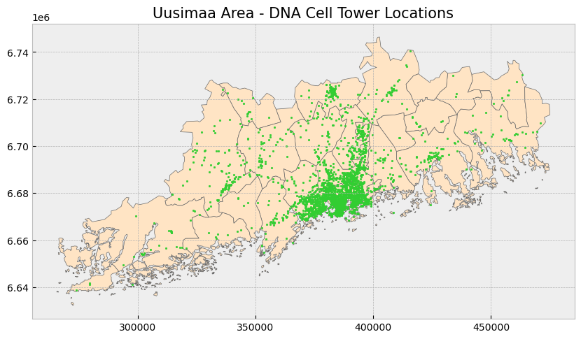
# Create subplots
fig, ax = plt.subplots(1, 1, figsize = (10, 10))

# Stylize plots
plt.style.use('bmh')

# Plot data
uusimaa_municipality.plot(ax = ax, color = 'bisque', edgecolor = 'dimgray')
uusimaa.plot(ax = ax, marker = 'o', color = 'limegreen', markersize = 3)

# Set title
ax.set_title('Uusimaa Area - DNA Cell Tower Locations', fontdict = {'fontsize': '15', 'fontweight' : '3'})

Text(0.5, 1.0, 'Uusimaa Area - DNA Cell Tower Locations')

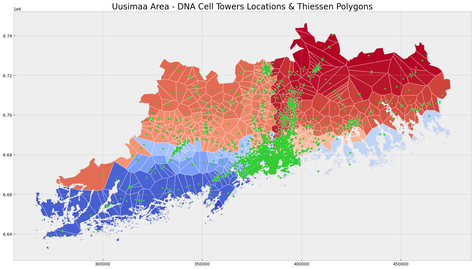
Thiessen Polygons

When creating Thiessen polygons, the sample points toward the edges of the point shapefile’s extent will have infinite Voronoi regions, because not all sides of these edge points have adjacent sample points that would constrain the regions. Consequently, these infinite regions will not be exported. To mitigate this issue, we can create dummy points well beyond the extent of our datasets, which will create finite Voronoi regions for all of our actual sample points. Then, we can clip the regions to our extent shapefile (creating dummy points far away from our actual sample points will ensure the dummy points and their infinite Voronoi regions do not interfere with the sample points and their associated finite Voronoi regions after all regions are clipped).

reference

from scipy.spatial import Voronoi, voronoi_plot_2d
from shapely.geometry import Polygon

# Get X and Y coordinates of cell towers
x = uusimaa_cell["geometry"].x
y = uusimaa_cell["geometry"].y

# Create list of XY coordinate pairs
coords = [list(xy) for xy in zip(x, y)]

# extend extent of municipality feature by using buffer
uusimaa_municipality_buffer = uusimaa_municipality.buffer(100000)

# get extent of buffered input feature
min_x_tp, min_y_tp, max_x_tp, max_y_tp = uusimaa_municipality_buffer.total_bounds

# use extent to create dummy points and add them to list of coordinates
coords_tp = coords + [[min_x_tp, min_y_tp], [max_x_tp, min_y_tp],
                    [max_x_tp, max_y_tp], [min_x_tp, max_y_tp]]

# calculate Voronoi diagram
tp = Voronoi(coords_tp)

# create empty list of hold Voronoi polygons
tp_poly_list = []

# create a polygon for each region
# 'regions' attribute provides a list of indices of the vertices (in the 'vertices' attribute) that make up the region
# Source: https://docs.scipy.org/doc/scipy/reference/generated/scipy.spatial.Voronoi.html
for region in tp.regions:
    # Ignore region if -1 is in the list (based on documentation)
    if -1 in region:
        continue
    else:
        pass
    
    if len(region) != 0:
        # Create a polygon by using the region list to call the correct elements in the 'vertices' attribute
        tp_poly_region = Polygon(list(tp.vertices[region]))
        tp_poly_list.append(tp_poly_region)
    else:
        continue
        
# create GeoDataFrame from list of polygon regions
tp_polys = gpd.GeoDataFrame(tp_poly_list, columns=['geometry'], crs=uusimaa_municipality.crs)

# Clip polygon regions to the municipality boundary
tp_polys_clipped = gpd.clip(tp_polys, uusimaa_municipality)

# Create subplots
fig, ax = plt.subplots(1, 1, figsize = (20, 20))

# Stylize plots
plt.style.use('bmh')

# Plot data
uusimaa_municipality.plot(ax = ax, color = 'none', edgecolor = 'dimgray')
tp_polys_clipped.plot(ax = ax, cmap = 'coolwarm', edgecolor = 'white', linewidth = 0.5)
uusimaa_cell.plot(ax = ax, marker = 'o', color = 'limegreen', markersize = 15)

# Set title
ax.set_title('Uusimaa Area - DNA Cell Towers Locations & Thiessen Polygons', fontdict = {'fontsize': '20', 'fontweight' : '3'})

Text(0.5, 1.0, 'Uusimaa Area - DNA Cell Towers Locations & Thiessen Polygons')

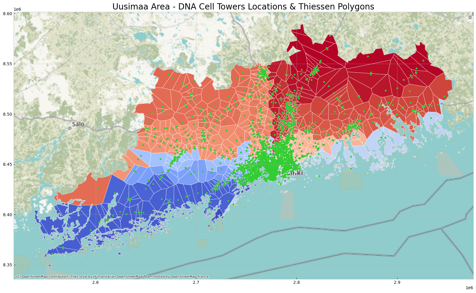
# change coordinates system
uusimaa_municipality_new = uusimaa_municipality.to_crs(epsg=3857)
tp_polys_clipped_new = tp_polys_clipped.to_crs(epsg=3857)
uusimaa_cell_new = uusimaa_cell.to_crs(epsg=3857)

# plot data
ax_new = uusimaa_municipality_new.plot(figsize=(20,20), color = 'none', edgecolor = 'dimgray')
tp_polys_clipped_new.plot(ax = ax_new, cmap = 'coolwarm', edgecolor = 'white', linewidth = 0.5)
uusimaa_cell_new.plot(ax = ax_new, marker = 'o', color = 'limegreen', markersize = 15)

# add background tiles to plot
ctx.add_basemap(ax_new)

# Set title
ax_new.set_title('Uusimaa Area - DNA Cell Towers Locations & Thiessen Polygons', fontdict = {'fontsize': '20', 'fontweight' : '3'})

Text(0.5, 1.0, 'Uusimaa Area - DNA Cell Towers Locations & Thiessen Polygons')