Geospatial interpolation - K-nearest neighbors

K-Nearest Neighbors (short as KNN) is a neighbor-based learning method that can be used for interpolation, in this case KNN looks for a specified number k of sampled points closests to an unknown point.

In this article, we have tried the following two applications by KNN algorithm:

• BallTree
• KNN regressor

BallTree is a space partitioning data structure for organizing points in a multi-dimensional space. A most common application of ball tree is for nearest neighbor search, the algorithm exploits the distance property of the ball tree. With this method, the unknown point is interpolated by the k nearest neighbors’ value (in our case is the measurement of 5G signal), a weighted method based on the distance (inverse distance weighting) is used as closer points have larger weight when deciding the unknown point’s value.

KNN regressor can be achieved by using sklearn library, the target (the unknow point) is predicted by local interpolation of the targets associated of the nearest neighbors.

Data Preparation

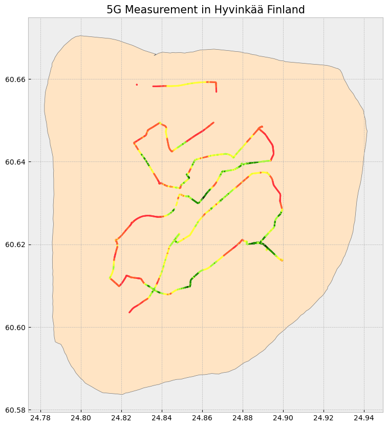
The 5G measurement is done by a 5G capable phone which could record the 5G serving cell information and signal quality information during the drive test, including physical cell ID, frequency, received signal strength (RSRP, RSRQ and SINR) etc. This measurement is an evidence of the network coverage and quality, but normally it cannot cover the every corner, therefore data interpolation is needed.

Geopandas can also read KML file, therefore it is possible to use geopandas to process the selv-defined polygons from Google Earth, refer references from Link 1 and Link 2.

import pandas as pd
import numpy as np
import geopandas as gpd
import matplotlib.pyplot as plt
from geopandas import GeoDataFrame
from shapely.geometry import Point
import geopy.distance
from sklearn.neighbors import BallTree
import warnings
warnings.filterwarnings('ignore')

# load 5G measurements
measurement_5g = pd.read_csv('5G Serving Cell.csv')

# create a GeoDataFrame with each measurement as a Point
measurement_5g_gdf = gpd.GeoDataFrame(measurement_5g, geometry=gpd.points_from_xy(measurement_5g['Longitude'], measurement_5g['Latitude'], crs='EPSG:4326'))

# import the polygon created from Google Earth
gpd.io.file.fiona.drvsupport.supported_drivers['KML'] = 'rw'
hyvinkaa = gpd.read_file('Hyvinkaa.kml', driver='KML')

def color_map(val):
    if val < -110:
        color = "#FF333C"
    elif val < -100:
        color = "#FF6133"
    elif val < -90:
        color = "#FFFF33"
    elif val < -80:
        color = "#A2FF33"
    elif val < -70:
        color = "#228E03"
    else:
        color = "#0E3B01"
    return color
measurement_5g_gdf['color'] = measurement_5g_gdf['RSRP(dBm)'].astype(float).map(color_map)

# Create subplots
fig, ax = plt.subplots(1, 1, figsize = (10, 10))

# Stylize plots
plt.style.use('bmh')

# Plot data
hyvinkaa.plot(ax = ax, color = 'bisque', edgecolor = 'dimgray')
measurement_5g_gdf.plot(ax = ax, marker = 'o', color = measurement_5g_gdf['color'], markersize = 3)

# Set title
ax.set_title('5G Measurement in Hyvinkää Finland', fontdict = {'fontsize': '15', 'fontweight' : '3'})

Text(0.5, 1.0, '5G Measurement in Hyvinkää Finland')

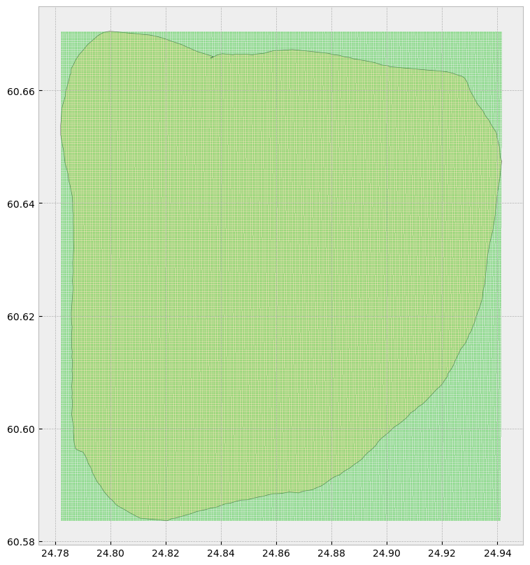
Build the Grid

To turn this data into a density map we will first need a grid. Then we can assign the 5G measurement value of the closest nearby property to each centroid.

# get extent of polygon's bounds
min_x_poly, min_y_poly, max_x_poly, max_y_poly = hyvinkaa.total_bounds

# create bounding box
LB = (min_y_poly,min_x_poly)  # Left Bottom
LT = (max_y_poly,min_x_poly)  # Left Top
RB = (min_y_poly,max_x_poly)  # Right Bottom
RT = (max_y_poly,max_x_poly)  # Right Top

# calculate the longitude distance and latitude distance
max_longitude_distance = geopy.distance.distance(LT,RT).km 
max_latitude_distance= geopy.distance.distance(RB,RT).km

# create the grid interval as 10 meters
longitude_interval = geopy.distance.distance(kilometers=0.01)

# calculate how many grids are need along longitude and latitude domain
grid=longitude_interval.km
n_longitude_grid_points = int(float(max_longitude_distance)/grid)
n_latitude_grid_points  = int(float(max_latitude_distance)/grid)
latitude_interval_degrees = (max_y_poly - min_y_poly)/n_latitude_grid_points

# greate a list of points
points = []

# build the grid
for j in range(n_latitude_grid_points): # Vertical 
    # start from bottom left (LB)
    start = (min_y_poly+(j*latitude_interval_degrees),min_x_poly)
    for i in range(n_longitude_grid_points): # Horizontal
        # Calculate the next point in the longitude direction 
        lon_offset = longitude_interval.destination(start, bearing=90). \
                      longitude - start[1]
        next_point = (start[0], start[1] + lon_offset)        
        points.append(next_point)        
        start = next_point

# Make a GeoDataFrame which will hold the grid
points = [(point[1], point[0]) for point in points]
points_gdf = [Point(point) for point in points] 
grid = gpd.GeoDataFrame(geometry=points_gdf, crs='epsg:4326')

# Create subplots
fig, ax = plt.subplots(1, 1, figsize = (10, 10))

# Stylize plots
plt.style.use('bmh')

# Plot data
hyvinkaa.plot(ax = ax, color = 'bisque', edgecolor = 'dimgray')
grid.plot(ax = ax, marker = 'o', color = 'limegreen', markersize = 0.005)

<Axes: >

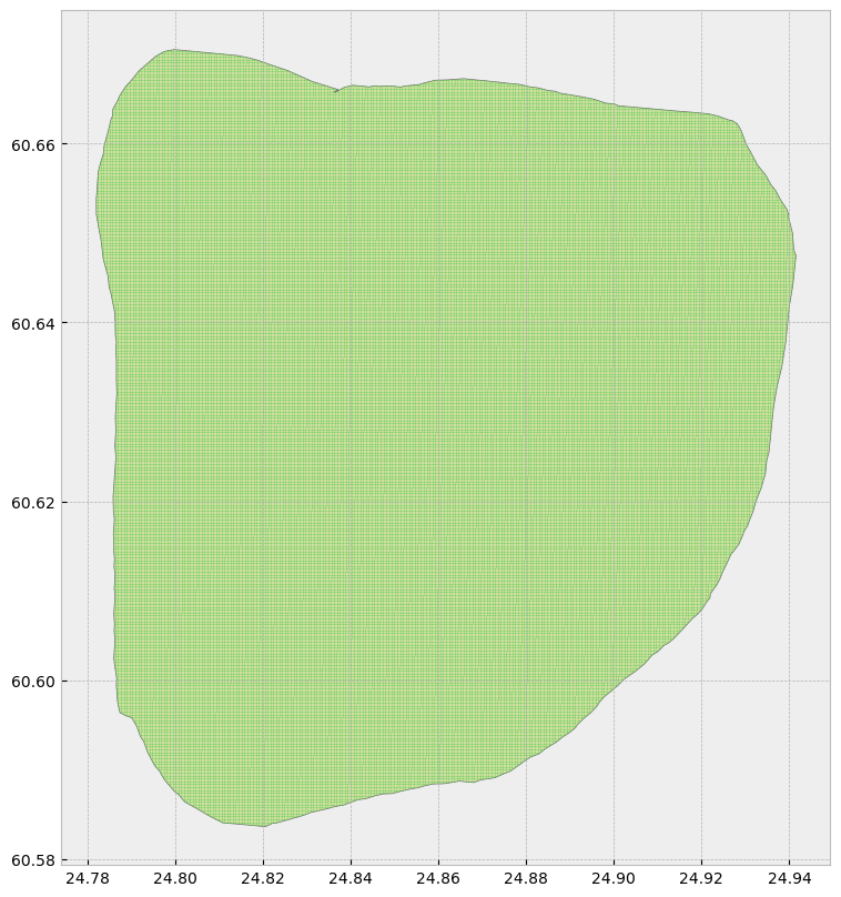
# Perform a spatial join between the two GeoDataFrames
joined = gpd.sjoin(grid, hyvinkaa, how='inner')

# Keep only the points inside the multipolygon
points_within_regions = joined['geometry']

# Create a new GeoDataFrame with only the points inside the multipolygon
grid_within_regions = gpd.GeoDataFrame(geometry=points_within_regions, crs='epsg:4326')

# Create subplots
fig, ax = plt.subplots(1, 1, figsize = (10, 10))

# Stylize plots
plt.style.use('bmh')

# Plot data
hyvinkaa.plot(ax = ax, color = 'bisque', edgecolor = 'dimgray')
grid_within_regions.plot(ax = ax, marker = 'o', color = 'limegreen', markersize = 0.005)

<Axes: >

K-Nearest Neighbors: BallTree

# Create a BallTree
tree = BallTree(measurement_5g_gdf['geometry'].apply(lambda p: [p.x, p.y]).tolist(),leaf_size=2)

# Query the BallTree on each centroid in 'grid_within_regions'
# to find the distance and id of 1 nearest neighbour in the 5G measurement
num_neighbors = 3 # The number of nearest neighbors
distances, indices = tree.query(
    grid_within_regions['geometry'].apply(lambda p: [p.x, p.y]).tolist(),
    k=num_neighbors)

measurement_array = np.array([[measurement_5g_gdf['RSRP(dBm)'].iloc[idx] for idx in row] for row in indices]) 
# Calculate the inverse of the distances
inverse_distances = 1 / distances

# Calculate the sum of the weights 
row_sum = np.sum(inverse_distances, axis=1).reshape(-1, 1)

# Normalize each row 
normalized_weights = inverse_distances/ row_sum

# Multiply the measurements by the corresponding weights
weighted_measurement = normalized_weights * measurement_array

# The measurement will be the sum of their weighted values
idw_measurement = np.sum(weighted_measurement, axis=1)

# Assign the measurement to the grid
grid_within_regions['5G RSRP(dBm)']= idw_measurement

Visualize the Results

The 5G coverage prediction in the center area could be more trustworthy as we have more measurement samples there, while on the boarder area, due to unsufficient number of samples, the prediction doesn’t look good.

# Plot the results

from matplotlib.colors import LinearSegmentedColormap
import contextily as ctx

color_palette=np.array([(215,24,29), (238,248,185), (41,130,185)])
color_palette=color_palette/255

cmap = LinearSegmentedColormap.from_list('5G RSRP(dBm)', color_palette) 

grid_within_regions = grid_within_regions.to_crs(epsg=3857)
ax = grid_within_regions.plot(column='5G RSRP(dBm)',figsize=(25, 15),alpha=0.5,legend=True,cmap=cmap, k=10)
ctx.add_basemap(ax)
plt.title('DNA 5G Coverage in Hyvinkää Finland using KNN BallTree',fontsize=20)
plt.show()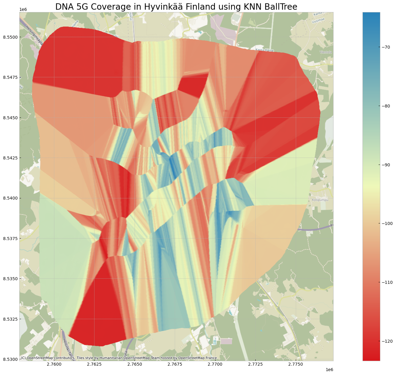

K-Nearest Neighbor Regressor

Using KDTree as the neighbor search algorithm, available choices are: ‘auto’, ‘ball_tree’, ‘kd_tree’, ‘brute’

from sklearn.neighbors import KNeighborsRegressor

# Get X and Y coordinates of measurement points and grid centroids
grid_within_regions = grid_within_regions.to_crs(epsg=4326)
x_meas = measurement_5g_gdf["geometry"].x
y_meas = measurement_5g_gdf["geometry"].y
x_grid = grid_within_regions['geometry'].x
y_grid = grid_within_regions['geometry'].y

# Create list of XY coordinate pairs
coords_meas = [list(xy) for xy in zip(x_meas, y_meas)]
coords_grid = [list(xy) for xy in zip(x_grid, y_grid)]

# Create a KNeighborsRegressor instance with the desired number of neighbors
knn_regressor = KNeighborsRegressor(n_neighbors=3, algorithm='kd_tree', weights='distance')

# Fit the KNeighborsRegressor to the input points and weights
knn_regressor.fit(coords, list(measurement_5g_gdf['RSRP(dBm)']))

# Perform KNN interpolation
interpolated_weights = knn_regressor.predict(coords_grid) 

# assign the results to the grid
grid_within_regions['KNN 5G RSRP(dBm)'] = interpolated_weights

Visualize the Results

Similar as BallTree approach, more measurements are required for better prediction.

# Plot the results

grid_within_regions = grid_within_regions.to_crs(epsg=3857)
ax = grid_within_regions.plot(column='KNN 5G RSRP(dBm)',figsize=(25, 15),alpha=0.5,legend=True,cmap=cmap, k=10)
ctx.add_basemap(ax)
plt.title('DNA 5G Coverage in Hyvinkää Finland using KNN Regressor',fontsize=20)
plt.show()

Reference

https://medium.com/@francode77/interpolation-using-knn-and-idw-fe546d5fb9ae