Two-dimensional histograms help to visualize two-dimensional points by dividing them among two-dimensional bins.
hist2d: two-dimensional histogram
%matplotlib inline
import numpy as np
import matplotlib.pyplot as plt
plt.style.use('seaborn-whitegrid')
import warnings
warnings.filterwarnings('ignore')
# generate some data from a multivariate Gaussian distribution
rng = np.random.default_rng(1701)
data = rng.normal(size=1000)
mean = [0,0]
cov = [[1,1],[1,2]]
x,y = rng.multivariate_normal(mean, cov, 10000).T# plot the two-dimensional histogram
plt.hist2d(x,y,bins=20)
cb = plt.colorbar()
cb.set_label('counts in bin')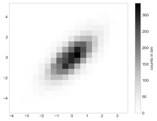
hexbin: hexagonal binnings
plt.hexbin(x,y, gridsize=30)
cb = plt.colorbar(label='count in bin')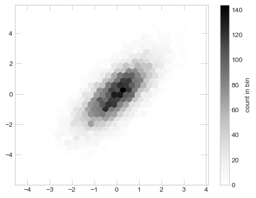
Kernel density estimation
Kernel density estimation could be used to “smear out” the points in space and add up the result to obtain a smooth function. scipy.stats provide a simple KDE implementation.
from scipy.stats import gaussian_kde

# fit an array of size [Ndim, Nsamples]
data = np.vstack([x,y])
kde = gaussian_kde(data)

# evaluate on a regular grid
xgrid = np.linspace(-3.5, 3.5, 40)
ygrid = np.linspace(-6, 6, 40)
Xgrid, Ygrid = np.meshgrid(xgrid, ygrid)
Z =kde.evaluate(np.vstack([Xgrid.ravel(), Ygrid.ravel()]))

# plot the result as an image
plt.imshow(Z.reshape(Xgrid.shape), origin='lower', aspect='auto', extent=[-3.5,3.5,-6,6])
cb = plt.colorbar()
cb.set_label('density')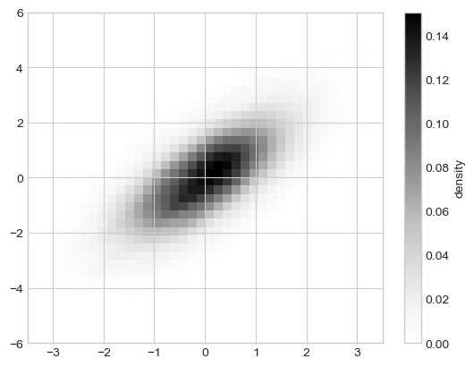
Reference
Python Data Science Handbook - Jake VanderPlas