Technical indicators Bollinger Bands

Background

Bollinger Bands are a type of statistical chart characterizing the prices and volatility over time of an asset, using a formulaic method propounded by John Bollinger in the 1980s.

Bollinger Bands consist of an N-period moving average (MA), an upper band at K times an N-period standard deviation above the moving average (MA + Kσ), and a lower band at K times an N-period standard deviation below the moving average (MA − Kσ). Typical values for N and K are 20 days and 2, respectively.

Bollinger Bands can be used to provide a relative definition of high and low prices of a market, that is to say, prices are high at the upper band and low at the lower band. Traders often use Bollinger Bands to determine whether an asset is overbought or oversold. When prices approach the upper band, it suggests that the asset may be overbought and due for a correction, while prices near the lower band suggest that the asset may be oversold and due for a rebound.

Python Implementation

import pandas as pd
import sqlite3

# load S&P500 data from stored database
sp500_db = sqlite3.connect(database="sp500_data.sqlite")

df = pd.read_sql_query(sql="SELECT * FROM SP500",
                       con=sp500_db,
                       parse_dates={"Date"})
df.head()

	level_0	index	Date	Ticker	Adj Close	Close	High	Low	Open	Volume	garmin_klass_vol	rsi
0	0	0	2014-04-29	A	35.049534	38.125893	38.304722	37.174534	38.118740	4688612.0	-0.002274	NaN
1	1	1	2014-04-29	AAL	33.476742	35.509998	35.650002	34.970001	35.200001	8994200.0	-0.000788	NaN
2	2	2	2014-04-29	AAPL	18.633333	21.154642	21.285000	21.053928	21.205000	337377600.0	-0.006397	NaN
3	3	3	2014-04-29	ABBV	34.034985	51.369999	51.529999	50.759998	50.939999	5601300.0	-0.062705	NaN
4	4	4	2014-04-29	ABT	31.831518	38.540001	38.720001	38.259998	38.369999	4415600.0	-0.013411	NaN

import pandas_ta
import numpy as np

# calculate bollinger bands for AAPL
aapl = df[df['Ticker'] == 'AAPL'].set_index('Date').drop('index',axis=1).drop('level_0',axis=1)
aapl['bb_low'] = pandas_ta.bbands(close=aapl['Adj Close'], length=20).iloc[:,0]
aapl['bb_mid'] = pandas_ta.bbands(close=aapl['Adj Close'], length=20).iloc[:,1]
aapl['bb_high'] = pandas_ta.bbands(close=aapl['Adj Close'], length=20).iloc[:,2]
aapl.tail()

	Ticker	Adj Close	Close	High	Low	Open	Volume	garmin_klass_vol	rsi	bb_low	bb_mid	bb_high
Date
2024-04-19	AAPL	165.000000	165.000000	166.399994	164.080002	166.210007	67772100.0	0.000078	37.902497	164.869819	170.207500	175.545180
2024-04-22	AAPL	165.839996	165.839996	167.259995	164.770004	165.520004	48116400.0	0.000111	39.784337	164.314856	169.885500	175.456143
2024-04-23	AAPL	166.899994	166.899994	167.050003	164.919998	165.350006	49537800.0	0.000049	42.166124	163.989522	169.687999	175.386475
2024-04-24	AAPL	169.020004	169.020004	169.300003	166.210007	166.539993	48251800.0	0.000085	46.706439	163.947623	169.653499	175.359375
2024-04-25	AAPL	169.889999	169.889999	170.610001	168.149994	169.529999	50558300.0	0.000104	48.493460	164.025646	169.482499	174.939352

import plotly.graph_objs as go
from datetime import datetime

# only select the data from 2023-01-01
aapl_new = aapl[aapl.index > datetime(2023,1,1)]

# Create a Plotly figure
fig = go.Figure()

# Add the price chart
fig.add_trace(go.Scatter(x=aapl_new.index, y=aapl_new['Adj Close'], mode='lines', name='Adj Close Price'))

# Add the Upper Bollinger Band and shade the area
fig.add_trace(go.Scatter(x=aapl_new.index, y=aapl_new['bb_high'], mode='lines', name='Upper Bollinger Band', line=dict(color='red')))
fig.add_trace(go.Scatter(x=aapl_new.index, y=aapl_new['bb_low'], fill='tonexty', mode='lines', name='Lower Bollinger Band', line=dict(color='green')))

# Add the Middle Bollinger Band (MA)
fig.add_trace(go.Scatter(x=aapl_new.index, y=aapl_new['bb_mid'], mode='lines', name='Middle Bollinger Band', line=dict(color='blue')))

# Customize the chart layout
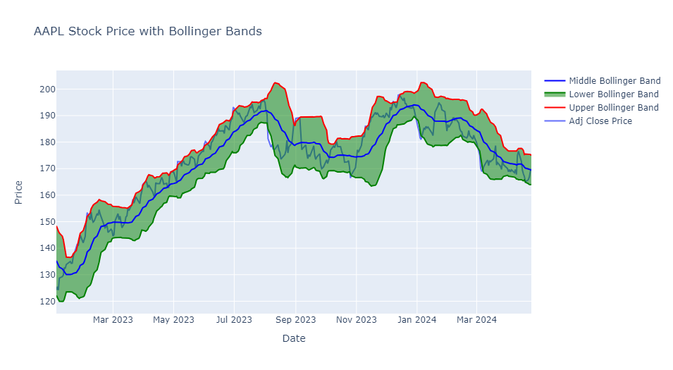
fig.update_layout(title='AAPL Stock Price with Bollinger Bands',
                  xaxis_title='Date',
                  yaxis_title='Price',
                  showlegend=True)

# Show the chart
fig.show()