Technical indicators Moving Averages

Background

A moving average is used to determine the direction of a trend, it sums up the data points of a financial security over a specific time period and divides the total by the number of data points to arrive at an average, this could help to smooth out the price data by creating a constantly updated average price.

By calculating the moving average, the impacts of random, short-term fluctuations on the price of a financial security over a specified time frame are mitigated.

Simple moving averages (SMAs)

The simple moving average (SMA) is straightforward and it is obtained by summing the recent data points in a given set and dividing the total by the number of time periods.

Exponential moving averages (EMAs)

Esponential moving agerage (EMA) gives more weight to the most recent price points to make it more responsive to recent data points.

Python Implementation

import pandas as pd
import sqlite3

# load S&P500 data from stored database
sp500_db = sqlite3.connect(database="sp500_data.sqlite")

df = pd.read_sql_query(sql="SELECT * FROM SP500",
                       con=sp500_db,
                       parse_dates={"Date"})
df.head()

	level_0	index	Date	Ticker	Adj Close	Close	High	Low	Open	Volume	garmin_klass_vol	rsi	atr	macd	macd signal	bb_low	bb_mid	bb_high
0	0	0	2014-04-29	A	35.049534	38.125893	38.304722	37.174534	38.118740	4688612.0	-0.002274	NaN	NaN	NaN	NaN	NaN	NaN	NaN
1	1	1	2014-04-29	AAL	33.476742	35.509998	35.650002	34.970001	35.200001	8994200.0	-0.000788	NaN	NaN	NaN	NaN	NaN	NaN	NaN
2	2	2	2014-04-29	AAPL	18.633333	21.154642	21.285000	21.053928	21.205000	337377600.0	-0.006397	NaN	NaN	NaN	NaN	NaN	NaN	NaN
3	3	3	2014-04-29	ABBV	34.034985	51.369999	51.529999	50.759998	50.939999	5601300.0	-0.062705	NaN	NaN	NaN	NaN	NaN	NaN	NaN
4	4	4	2014-04-29	ABT	31.831518	38.540001	38.720001	38.259998	38.369999	4415600.0	-0.013411	NaN	NaN	NaN	NaN	NaN	NaN	NaN

# remove irrelevant columns
df = df.drop('index', axis=1)
df = df.drop('level_0', axis=1)
df.head()

	Date	Ticker	Adj Close	Close	High	Low	Open	Volume	garmin_klass_vol	rsi	atr	macd	macd signal	bb_low	bb_mid	bb_high
0	2014-04-29	A	35.049534	38.125893	38.304722	37.174534	38.118740	4688612.0	-0.002274	NaN	NaN	NaN	NaN	NaN	NaN	NaN
1	2014-04-29	AAL	33.476742	35.509998	35.650002	34.970001	35.200001	8994200.0	-0.000788	NaN	NaN	NaN	NaN	NaN	NaN	NaN
2	2014-04-29	AAPL	18.633333	21.154642	21.285000	21.053928	21.205000	337377600.0	-0.006397	NaN	NaN	NaN	NaN	NaN	NaN	NaN
3	2014-04-29	ABBV	34.034985	51.369999	51.529999	50.759998	50.939999	5601300.0	-0.062705	NaN	NaN	NaN	NaN	NaN	NaN	NaN
4	2014-04-29	ABT	31.831518	38.540001	38.720001	38.259998	38.369999	4415600.0	-0.013411	NaN	NaN	NaN	NaN	NaN	NaN	NaN

import pandas_ta

df = df.set_index(['Date','Ticker'])
# compute SMA and EMA
df['sma'] = df.groupby(level=1)['Adj Close'].transform(lambda x: pandas_ta.sma(close=x,length=20))
df['ema'] = df.groupby(level=1)['Adj Close'].transform(lambda x: pandas_ta.ema(close=x,length=20))
df.tail()

		Adj Close	Close	High	Low	Open	Volume	garmin_klass_vol	rsi	atr	macd	macd signal	bb_low	bb_mid	bb_high	sma	ema
Date	Ticker
2024-04-25	XYL	130.610001	130.610001	131.199997	128.100006	129.619995	963600.0	0.000264	61.482745	0.665306	0.355146	0.255276	4.845591	4.863502	4.881413	128.482000	128.582695
	YUM	141.559998	141.559998	142.169998	140.389999	141.979996	1693100.0	0.000076	65.668163	0.322566	0.550830	0.285784	4.913482	4.937968	4.962454	138.497000	138.658563
	ZBH	119.750000	119.750000	121.349998	118.769997	120.709999	1078800.0	0.000206	35.636078	-0.350196	-0.889200	-0.646480	4.772846	4.835888	4.898931	125.012999	123.565569
	ZBRA	292.529999	292.529999	293.290009	271.630005	274.359985	674700.0	0.001355	56.172272	0.500501	-0.391439	-0.242456	5.588730	5.666387	5.744044	288.205502	284.262362
	ZTS	153.360001	153.360001	153.589996	150.039993	150.970001	4567200.0	0.000178	39.809619	1.374957	-3.202379	-3.584353	4.967408	5.065065	5.162723	157.579352	157.003521

# update the database
df = df.reset_index()
df.to_sql(name="SP500",
          con=sp500_db,
          if_exists="replace",
          index=True)
sp500_db.close()

import plotly.graph_objs as go
from datetime import datetime

# select AAPL
aapl = df[df['Ticker'] == 'AAPL'].set_index('Date')

# only select the data from 2023-01-01
aapl_new = aapl[aapl.index > datetime(2023,1,1)]

# create a Plotly figure
fig = go.Figure()

# add the price chart
fig.add_trace(go.Scatter(x=aapl_new.index, y=aapl_new['Adj Close'], mode='lines', name='Adj Close Price'))

# add the SMA chart
fig.add_trace(go.Scatter(x=aapl_new.index, y=aapl_new['sma'], mode='lines', name='SMA'))

# add the EMA chart
fig.add_trace(go.Scatter(x=aapl_new.index, y=aapl_new['ema'], mode='lines', name='EMA'))

# Customize the chart layout
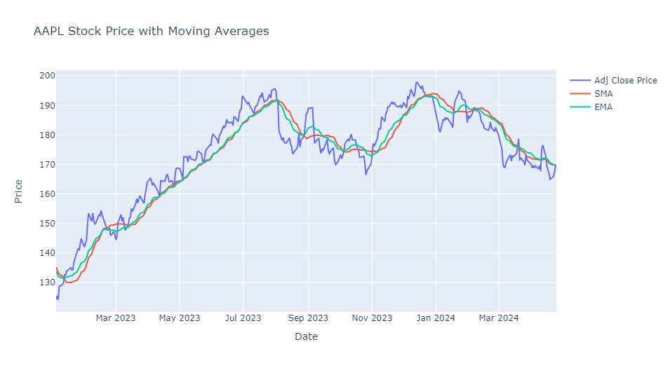
fig.update_layout(title='AAPL Stock Price with Moving Averages',
                  xaxis_title='Date',
                  yaxis_title='Price',
                  showlegend=True)

# Show the chart
fig.show()