Technical indicators Average True Range (ATR)

Background

The average true range (ATR) is a technical analysis indicator that measures market volatility by decomposing the entire range of an asset price for that period.

The true range indicator is taken as the greatest of the following: current high less the current low; the absolute value of the current high less the previous close; and the absolute value of the current low less the previous close. The ATR is then a moving average, generally using 14 days, of the true ranges.

For a higher ATR, it indicates the stock is experiencing a high level of volatility, in contrast that a lower ATR indicates lower volatility for the period evaluated. Therefore the ATR may be used to decide when to enter and exit trades and is a useful tool to add to a trading system.

Chuck LeBeau developed a popular technique using ATR to make exit decision called “chandelier exit”, it places a trailing stop under the highest high the stock has reached since you entered the trade.

The main limitations of using ATR as an indicator are it is a subjective measure therefore it is open to interpretation, which means a single ATR value could not tell you with any certainty that a trend is about to reverse or not. It needs to be compared against earlier readings to review a trend’s strength or weakness. Another limitation is the ATR only measures volatility and not the direction of an asset’s price.

A normal ATR is 1.18, if it is much higher or lower than this alue, it might indicate that further investigation is required.

Python Implementation

import pandas as pd
import sqlite3

# load S&P500 data from stored database
sp500_db = sqlite3.connect(database="sp500_data.sqlite")

df = pd.read_sql_query(sql="SELECT * FROM SP500",
                       con=sp500_db,
                       parse_dates={"Date"})
df.head()

	level_0	index	Date	Ticker	Adj Close	Close	High	Low	Open	Volume	garmin_klass_vol	rsi
0	0	0	2014-04-29	A	35.049534	38.125893	38.304722	37.174534	38.118740	4688612.0	-0.002274	NaN
1	1	1	2014-04-29	AAL	33.476742	35.509998	35.650002	34.970001	35.200001	8994200.0	-0.000788	NaN
2	2	2	2014-04-29	AAPL	18.633333	21.154642	21.285000	21.053928	21.205000	337377600.0	-0.006397	NaN
3	3	3	2014-04-29	ABBV	34.034985	51.369999	51.529999	50.759998	50.939999	5601300.0	-0.062705	NaN
4	4	4	2014-04-29	ABT	31.831518	38.540001	38.720001	38.259998	38.369999	4415600.0	-0.013411	NaN

# remove irrelevant columns
df = df.drop('level_0', axis=1)
df = df.drop('index', axis=1)
df.head()

	Date	Ticker	Adj Close	Close	High	Low	Open	Volume	garmin_klass_vol	rsi
0	2014-04-29	A	35.049534	38.125893	38.304722	37.174534	38.118740	4688612.0	-0.002274	NaN
1	2014-04-29	AAL	33.476742	35.509998	35.650002	34.970001	35.200001	8994200.0	-0.000788	NaN
2	2014-04-29	AAPL	18.633333	21.154642	21.285000	21.053928	21.205000	337377600.0	-0.006397	NaN
3	2014-04-29	ABBV	34.034985	51.369999	51.529999	50.759998	50.939999	5601300.0	-0.062705	NaN
4	2014-04-29	ABT	31.831518	38.540001	38.720001	38.259998	38.369999	4415600.0	-0.013411	NaN

import pandas_ta

# calculate ATR
def compute_atr(stock_data):
    atr = pandas_ta.atr(high=stock_data['High'],
                        low=stock_data['Low'],
                        close=stock_data['Close'],
                        length=14)
    return atr.sub(atr.mean()).div(atr.std())

df = df.set_index(['Date','Ticker'])
df['atr'] = df.groupby(level=1, group_keys=False).apply(compute_atr)
df.tail()

		Adj Close	Close	High	Low	Open	Volume	garmin_klass_vol	rsi	atr
Date	Ticker
2024-04-25	XYL	130.610001	130.610001	131.199997	128.100006	129.619995	963600.0	0.000264	61.482745	0.665306
	YUM	141.559998	141.559998	142.169998	140.389999	141.979996	1693100.0	0.000076	65.668163	0.322566
	ZBH	119.750000	119.750000	121.349998	118.769997	120.709999	1078800.0	0.000206	35.636078	-0.350196
	ZBRA	292.529999	292.529999	293.290009	271.630005	274.359985	674700.0	0.001355	56.172272	0.500501
	ZTS	153.360001	153.360001	153.589996	150.039993	150.970001	4567200.0	0.000178	39.809619	1.374957

# update the database
df = df.reset_index()
df.to_sql(name="SP500",
          con=sp500_db,
          if_exists="replace",
          index=True)
sp500_db.close()

import matplotlib.pyplot as plt
from datetime import datetime

# select AAPL
aapl = df[df['Ticker'] == 'AAPL'].set_index('Date')

# only select the data from 2022-01-01
aapl_new = aapl[aapl.index > datetime(2022,1,1)]

# set the theme of the chart
plt.style.use('fivethirtyeight')
plt.rcParams['figure.figsize'] = (20,16)

# create two charts on the same figure
ax1 = plt.subplot2grid((10,1),(0,0), rowspan=4, colspan=1)
ax2 = plt.subplot2grid((10,1),(5,0), rowspan=4, colspan=1)

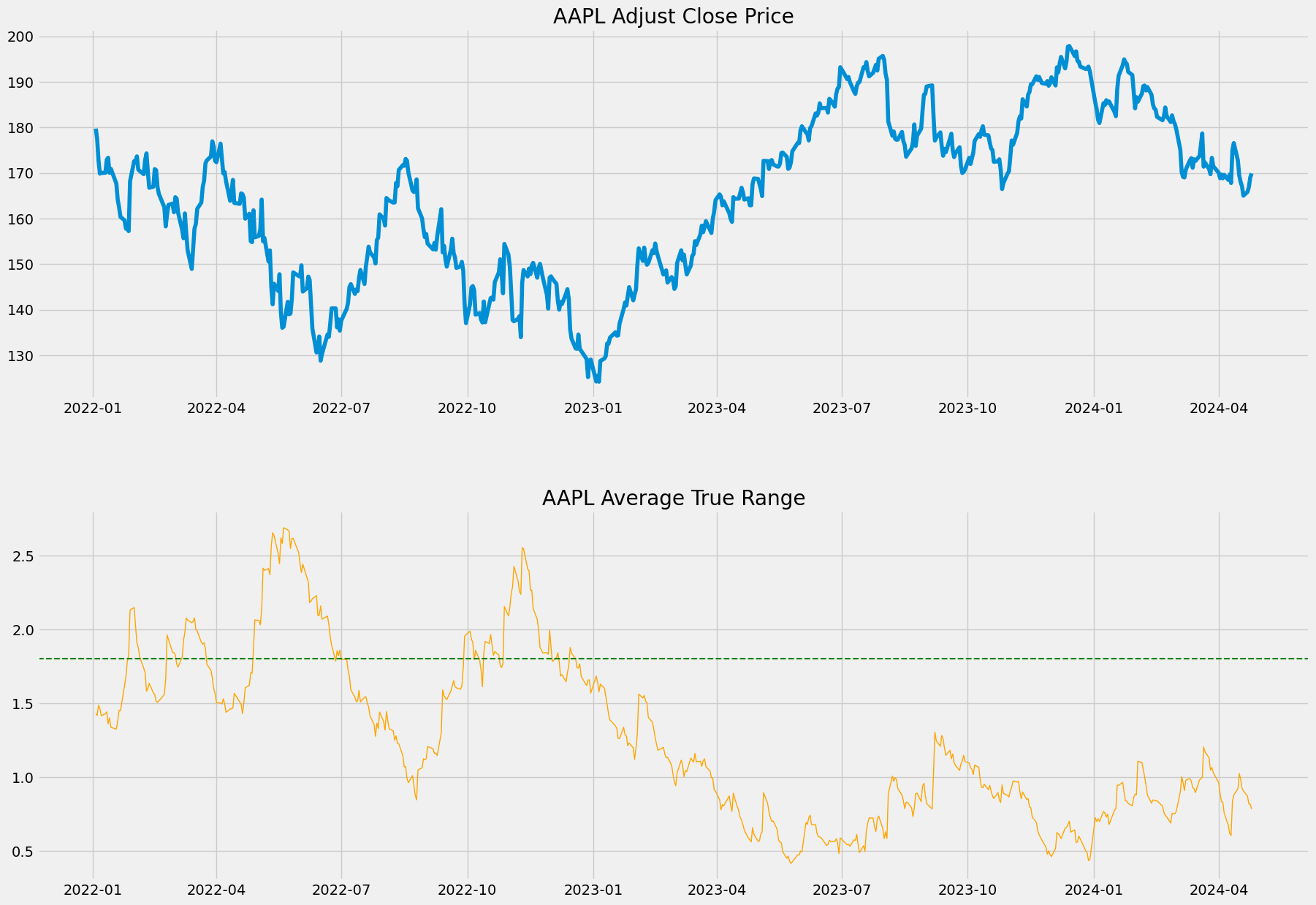
# plot the closing price on the first chart
ax1.plot(aapl_new['Adj Close'])
ax1.set_title('AAPL Adjust Close Price')

# plot the RSI on the second chart
ax2.plot(aapl_new['atr'], color='orange', linewidth=1)
ax2.set_title('AAPL Average True Range')

# add a horizontal line, signaling the normal ATR
ax2.axhline(1.8, linestyle='--', linewidth=1.5, color='green')

<matplotlib.lines.Line2D at 0x1ce20e36990>

Reference

Average True Range (ATR) Formula, What It Means, and How to Use It by Adam Hayes on Investopedia