Technical indicators Accumulation Distribution Indicator (AD)

Background

The accumulation/distribution indicator (A/D) is a cumulative indicator that uses volume and price to assess whether a stock is being accumulated or distributed. The A/D measure seeks to identify divergences between the stock price and the volume flow. It provides a measure of the commitment of bulls and bears to the market and is used to detect divergences between volume and price action - signs that a trend is weakening.

If the price is rising but the indicator is falling, then it suggests that buying or accumulation volume may not be enough to support the price rise and a price decline could be forthcoming.

The Accumulation/Distribution is calculated using the following formula: AD = AD + ((Close - Low) - (High - Close)) / (High - Low) * Volume

If a security’s price is in a downtrend while the A/D line is in an uptrend, then the indicator shows there may be buying pressure and the security’s price may reverse to the upside. Conversely, if a security’s price is in an uptrend while the A/D line is in a downtrend, then the indicator shows there may be selling pressure, or higher distribution. This warns that the price may be due for a decline.

Python Implementation

import pandas as pd
import sqlite3

# load S&P500 data from stored database
sp500_db = sqlite3.connect(database="sp500_data.sqlite")

df = pd.read_sql_query(sql="SELECT * FROM SP500",
                       con=sp500_db,
                       parse_dates={"Date"})
df.head()

	index	Date	Ticker	Adj Close	Close	High	Low	Open	Volume	garmin_klass_vol	rsi	atr	macd	macd signal	bb_low	bb_mid	bb_high	sma	ema
0	0	2014-04-29	A	35.049534	38.125893	38.304722	37.174534	38.118740	4688612.0	-0.002274	NaN	NaN	NaN	NaN	NaN	NaN	NaN	NaN	NaN
1	1	2014-04-29	AAL	33.476742	35.509998	35.650002	34.970001	35.200001	8994200.0	-0.000788	NaN	NaN	NaN	NaN	NaN	NaN	NaN	NaN	NaN
2	2	2014-04-29	AAPL	18.633333	21.154642	21.285000	21.053928	21.205000	337377600.0	-0.006397	NaN	NaN	NaN	NaN	NaN	NaN	NaN	NaN	NaN
3	3	2014-04-29	ABBV	34.034985	51.369999	51.529999	50.759998	50.939999	5601300.0	-0.062705	NaN	NaN	NaN	NaN	NaN	NaN	NaN	NaN	NaN
4	4	2014-04-29	ABT	31.831518	38.540001	38.720001	38.259998	38.369999	4415600.0	-0.013411	NaN	NaN	NaN	NaN	NaN	NaN	NaN	NaN	NaN

# remove irrelevant columns
df = df.drop('index', axis=1)
#df = df.drop('level_0', axis=1)
df.head()

	Date	Ticker	Adj Close	Close	High	Low	Open	Volume	garmin_klass_vol	rsi	atr	macd	macd signal	bb_low	bb_mid	bb_high	sma	ema
0	2014-04-29	A	35.049534	38.125893	38.304722	37.174534	38.118740	4688612.0	-0.002274	NaN	NaN	NaN	NaN	NaN	NaN	NaN	NaN	NaN
1	2014-04-29	AAL	33.476742	35.509998	35.650002	34.970001	35.200001	8994200.0	-0.000788	NaN	NaN	NaN	NaN	NaN	NaN	NaN	NaN	NaN
2	2014-04-29	AAPL	18.633333	21.154642	21.285000	21.053928	21.205000	337377600.0	-0.006397	NaN	NaN	NaN	NaN	NaN	NaN	NaN	NaN	NaN
3	2014-04-29	ABBV	34.034985	51.369999	51.529999	50.759998	50.939999	5601300.0	-0.062705	NaN	NaN	NaN	NaN	NaN	NaN	NaN	NaN	NaN
4	2014-04-29	ABT	31.831518	38.540001	38.720001	38.259998	38.369999	4415600.0	-0.013411	NaN	NaN	NaN	NaN	NaN	NaN	NaN	NaN	NaN

import pandas_ta

df = df.set_index(['Date','Ticker'])

# compute AD

def compute_ad(stock_data):
    ad = pandas_ta.ad(high=stock_data['High'],
                        low=stock_data['Low'],
                        close=stock_data['Close'],
                        volume=stock_data['Volume'],
                        length=14)
    return ad

df['ad'] = df_new.groupby(level=1, group_keys=False).apply(compute_ad)
df.tail()

		Adj Close	Close	High	Low	Open	Volume	garmin_klass_vol	rsi	atr	macd	macd signal	bb_low	bb_mid	bb_high	sma	ema	ad
Date	Ticker
2024-04-25	XYL	130.610001	130.610001	131.199997	128.100006	129.619995	963600.0	0.000264	61.482745	0.665306	0.355146	0.255276	4.845591	4.863502	4.881413	128.482000	128.582695	1.381747e+08
	YUM	141.559998	141.559998	142.169998	140.389999	141.979996	1693100.0	0.000076	65.668163	0.322566	0.550830	0.285784	4.913482	4.937968	4.962454	138.497000	138.658563	8.902989e+07
	ZBH	119.750000	119.750000	121.349998	118.769997	120.709999	1078800.0	0.000206	35.636078	-0.350196	-0.889200	-0.646480	4.772846	4.835888	4.898931	125.012999	123.565569	7.870077e+07
	ZBRA	292.529999	292.529999	293.290009	271.630005	274.359985	674700.0	0.001355	56.172272	0.500501	-0.391439	-0.242456	5.588730	5.666387	5.744044	288.205502	284.262362	5.349014e+07
	ZTS	153.360001	153.360001	153.589996	150.039993	150.970001	4567200.0	0.000178	39.809619	1.374957	-3.202379	-3.584353	4.967408	5.065065	5.162723	157.579352	157.003521	2.636284e+08

# update the database
df = df.reset_index()
df.to_sql(name="SP500",
          con=sp500_db,
          if_exists="replace",
          index=True)
sp500_db.close()

import matplotlib.pyplot as plt
from datetime import datetime

# select AAPL
aapl = df[df['Ticker'] == 'AAPL'].set_index('Date')

# only select the data from 2022-01-01
aapl_new = aapl[aapl.index > datetime(2022,1,1)]

# set the theme of the chart
plt.style.use('fivethirtyeight')
plt.rcParams['figure.figsize'] = (20,16)

# create two charts on the same figure
ax1 = plt.subplot2grid((10,1),(0,0), rowspan=4, colspan=1)
ax2 = plt.subplot2grid((10,1),(5,0), rowspan=4, colspan=1)

# plot the closing price on the first chart
ax1.plot(aapl_new['Adj Close'])
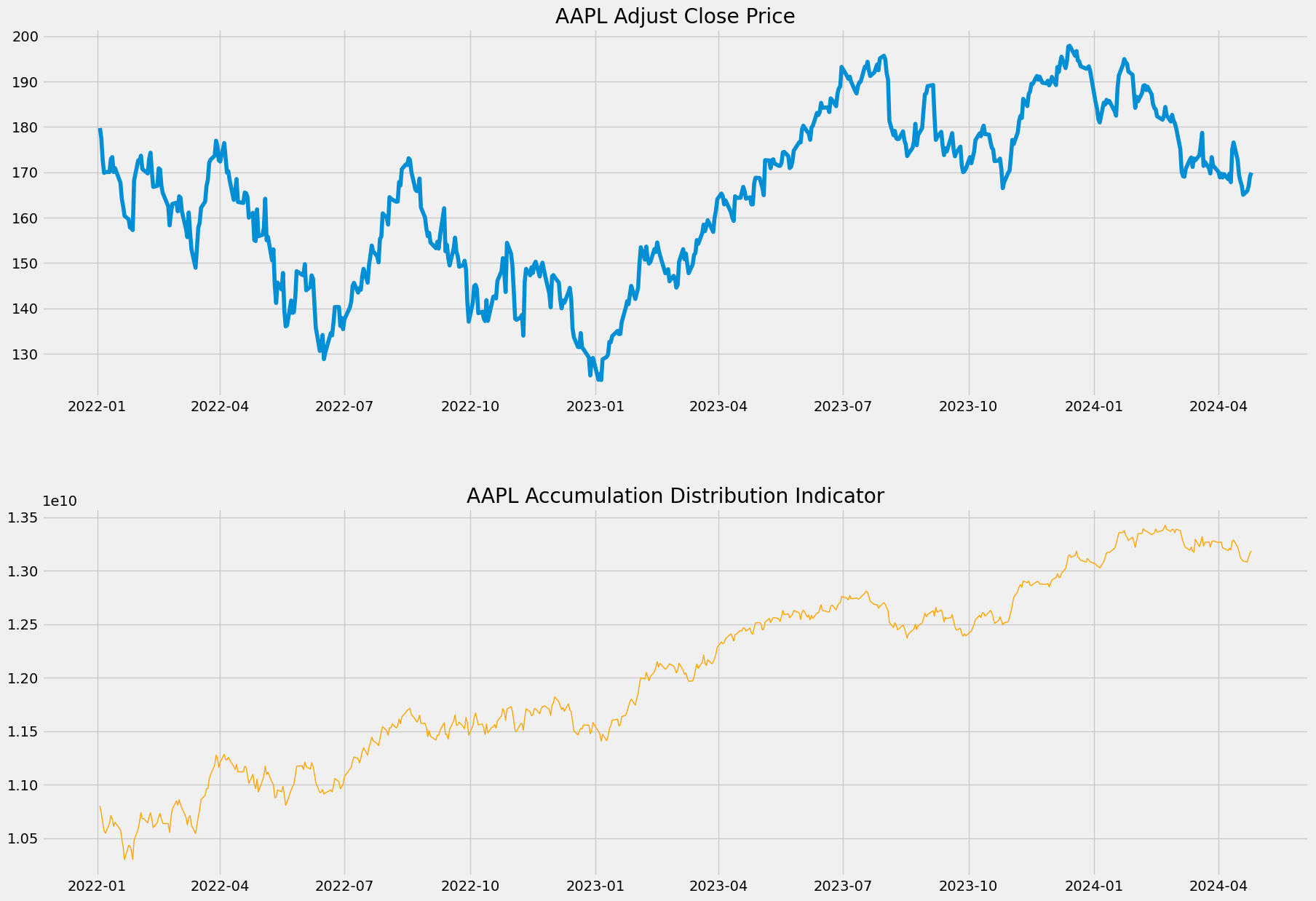
ax1.set_title('AAPL Adjust Close Price')

# plot the AD on the second chart
ax2.plot(aapl_new['ad'], color='orange', linewidth=1)
ax2.set_title('AAPL Accumulation Distribution Indicator')

Text(0.5, 1.0, 'AAPL Accumulation Distribution Indicator')

Reference

Accumulation/Distribution Indicator (A/D): What it Tells You by Cory Mitchell on Investopedia
e